EASY METHOD TO APPLY CONDITIONAL FORMATTING BASED ON TEXT IN EXCEL?

Table of Contents

• INTRODUCTION
• HOW TEXT IS HANDLED IN EXCEL?
• WHAT IS CONDITIONAL FORMATTING BASED ON TEXT IN EXCEL?
• EXAMPLE 1: HOW TO HIGHLIGHT THE TEXT EQUAL TO A GIVEN VALUE IN EXCEL USING CONDITIONAL FORMATTING BASED ON TEXT IN EXCEL ?
• EXAMPLE 2: HOW TO  HIGHLIGHT THE TEXT MATCHING THE GIVEN TEXT CASE SENSITIVE USING CONDITIONAL FORMATTING BASED ON TEXT IN EXCEL?
• EXAMPLE 3: HOW TO  HIGHLIGHT THE CELLS THAT CONTAIN A SPECIFIC TEXT USING CONDITIONAL FORMATTING BASED ON TEXT IN EXCEL
• EXAMPLE 4: HOW TO HIGHLIGHT THE VALUE SELECTED IN A DROPDOWN LIST USING CONDITIONAL FORMATTING BASED ON TEXT IN EXCEL
• SUGGESTED READS:

INTRODUCTION

In this article, we’ll be focussing on using conditional formatting based on text in Excel.

Whenever we prepare any report in excel, we have two constituents in report–The Text portion and the Numerical portion.

But just storing the text and numbers doesn’t make the super reports.

Many times we need to automate the process in the reports to minimize the effort and improve the accuracy.

Many functions are provided by Excel which works on Text and give us useful output as well without much effort. But a few problems are still left on which we need to apply some tricks with the available tools.

One of such condition is using conditional formatting based on text in Excel. Although a number of options are present but the situations outnumber them.

In this article, we will continue learning many more techniques about the manipulation of text in Excel.

FOR MORE INFORMATION ABOUT MANIPULATING TEXT, CLICK MANIPULATING TEXT IN EXCEL – PART I

HOW TEXT IS HANDLED IN EXCEL?

TEXT is simply the group of characters and strings of characters which convey the information about the different data and numbers in Excel. Every character is connected with a code [ANSI].

Text comprises of the individual entity character which is the smallest bit which would be found in Excel.

We can perform the operations on the strings[Text] or the characters. Characters are not limited to A to Z or a to z but many symbols are also included in this which we would see in the later part of the article. 

TEXT IS AN INACTIVE NUMBER TYPE[FORMAT] IN EXCEL. ANYTHING STORED AS TEXT [NUMBER OR DATE] WON’T RESPOND TO ANY STANDARD FORMULAS OR FUNCTIONS BUT SPECIALLY DESIGNED TEXT FUNCTIONS. [EXCEPTIONS DO OCCUR IN CASE OF NUMBERS]

If we need to make anything inactive, such as Date to be non-responding to the calculation, we put it as a text. Similarly, if we want to avoid any calculations for a number it needs to be put as a text.     

WHAT IS CONDITIONAL FORMATTING BASED ON TEXT IN EXCEL?

CONDITIONAL FORMATTING is the process of formatting the data in Excel on the basis of the conditions.

We can put many conditions in the cell and program the Excel to make the formatting, as desired if the particular condition is met. Formatting comprises of the foreground color, background color, font, size etc. which are the properties of the text.

It makes the results more readable.

IT IS RECOMMENDED TO LEARN THE BASICS OF CONDITIONAL FORMATTING BEFORE YOU LEARN THE CONDITIONAL FORMATTING BASED ON TEXT IN EXCEL.

CLICK HERE TO LEARN ABOUT CONDITIONAL FORMATTING.

Maximum times, we apply the conditional formatting on the basis of values present in the cells.

Let us now learn the way by which we can apply conditional formatting based on text in Excel.

EXAMPLES SHOWING CONDITIONAL FORMATTING BASED ON TEXT IN EXCEL.

EXAMPLE 1: HOW TO HIGHLIGHT THE TEXT EQUAL TO A GIVEN VALUE IN EXCEL USING CONDITIONAL FORMATTING BASED ON TEXT IN EXCEL ?

Let us find out the cell which contains a text value equal to some SPECIFIED TEXT.

For the example let us take this block of text values in Excel.

HELLO	HOW	ARE	YOU	RED
GREEN	YELLOW	BLUE	GREY	WHITE
BIG	BUFFALO	ZEBRA	XYLOPHONE	SMALL
BLACK	APPLE	MANGO	GUAVA	ONION
PUMPKIN	OKRA	KIWI	POTATO	SPRING

 Let us try to highlight the cells containing HELLO.

It can be done in two ways.

1. Using the predefined options.

2. Using custom formula.

1. USING PREDEFINED OPTIONS

 STEPS to highlight cells using the predefined option:

1.  Select the complete table.
2. Go to HOME TAB>CONDITIONAL FORMATTING>HIGHLIGHT CELL RULES>EQUAL TO

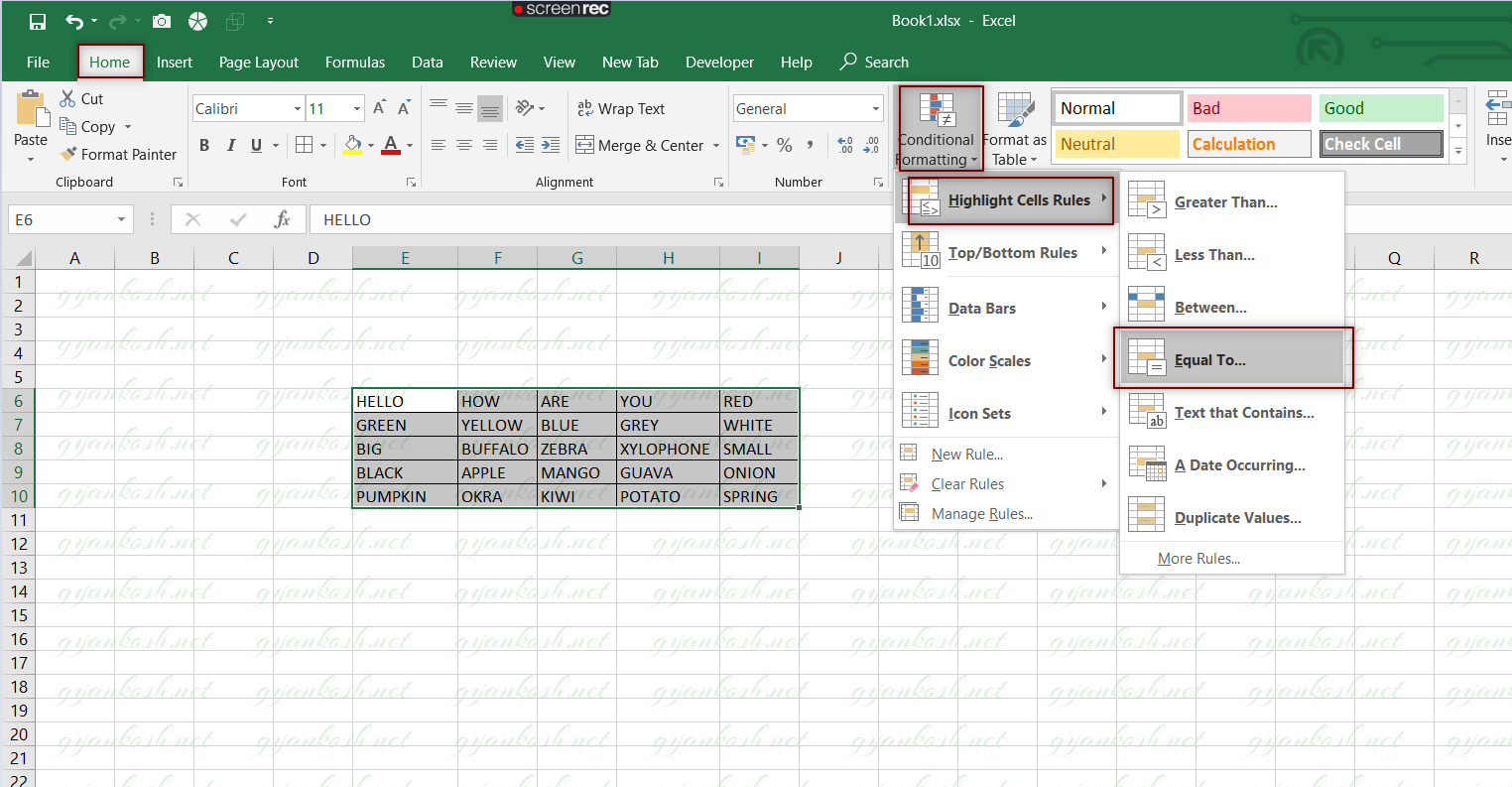
3. Click EQUAL TO.
4. The following dialog box will open.
5. Enter the value in the field as shown in the picture.
6. Select the format of the cells which satisfy the condition.
7. and Click OK.

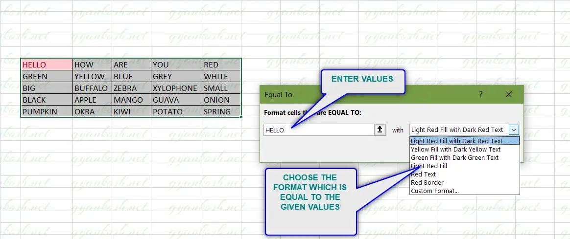
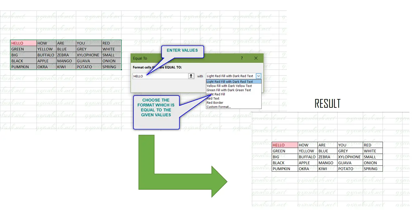
• After clicking OK, we will see the result as the cell with HELLO will be in pink. [The option doesn’t differ the cases. Both of upper and lower cases will be taken as same.]
• Similarly we can find other values too.

2. USING CUSTOM FORMULA

 STEPS to highlight cells using the custom formula:

1.  Select the complete table.
2. Go to HOME TAB>CONDITIONAL FORMATTING>NEW RULE.
3. A dialog box as shown in the picture below will open.
4. Click the last option: use a formula to determine which cells to format.

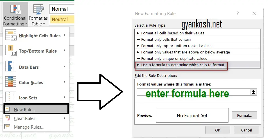
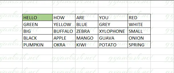
5.  Enter the formula in the field as =E6=”HELLO”.
6. Set the format as per your choice. We set the fill color as green.[Don’t forget to change the format otherwise difference won’t be visible.]
7. Click OK.
8. The result will be highlighted as shown in the picture below.

For the concept OF CONDITIONAL FORMATTING CLICK HERE.

EXAMPLE 2: HOW TO HIGHLIGHT THE TEXT MATCHING THE GIVEN TEXT CASE SENSITIVE USING CONDITIONAL FORMATTING BASED ON TEXT IN EXCEL?

In this example, let us find out the way to highlight the cells which contain the text same as some specified text exactly with the same content and with the same case. 

In this example, we are taking a table of data for highlighting the text which satisfies the condition given.

We can also apply the same method to highlight the exact text using conditional formatting for the given List of different data.

GENERALIZED FORMULA TO HIGHLIGHT THE EXACT TEXT:

=EXACT(FIRST CELL OF SELECTION, “TEXT TO BE MATCHED”).

For our example, we will highlight the cell containing the text “Yellow”. Follow the steps.

1. Select the complete table.
2. Go to HOME TAB>CONDITIONAL FORMATTING>NEW RULE.
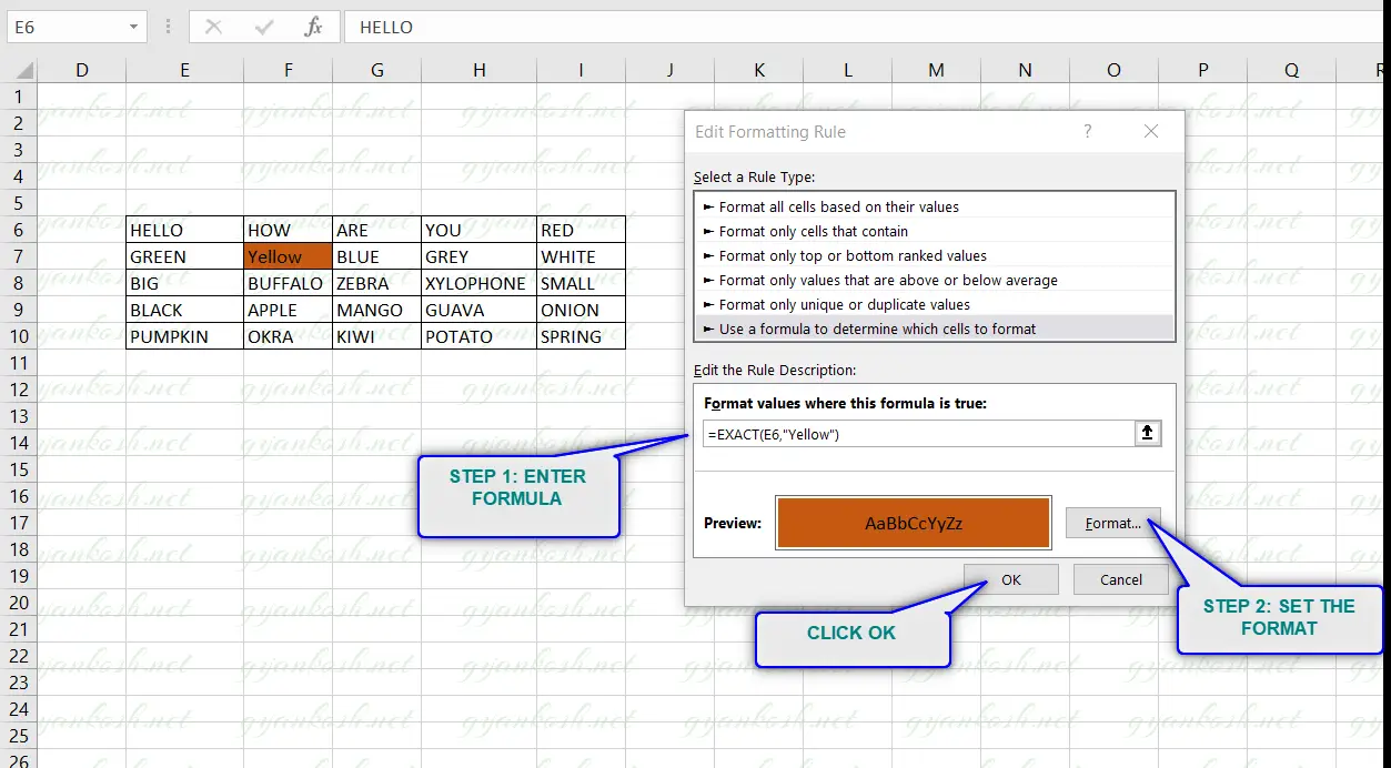
3. A dialog box as shown in the picture below will open.
4. Click the last option: use a formula to determine which cells to format.
5. Enter the formula =EXACT(E6,”Yellow”).
6. Choose the format of your choice, which will appear when some cell fulfill the condition.
7. Click OK.

For the concept OF CONDITIONAL FORMATTING CLICK HERE.

EXAMPLE 3: HOW TO HIGHLIGHT THE CELLS THAT CONTAIN A SPECIFIC TEXT USING CONDITIONAL FORMATTING BASED ON TEXT IN EXCEL

Suppose we want to create a condition when we want to highlight the cell if the cell contains any specific character say # for our example.

GENERALIZED FORMULA TO HIGHLIGHT THE CELLS WHICH CONTAIN A SPECIFIC TEXT ( ANY SMALLER STRING)

1. Select the complete table.
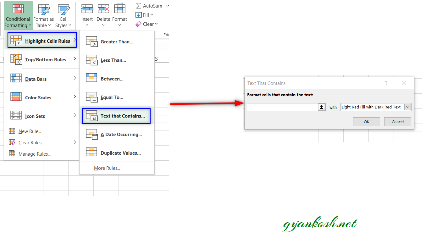
2. Go to HOME TAB>CONDITIONAL FORMATTING>HIGHLIGHT CELLS RULES.
3. Enter the character in the field.
4. Choose the FORMAT as you require the result to be.
5. Click OK.

For the concept of CONDITIONAL FORMATTING CLICK HERE.


UPDATE 1

EXAMPLE 4: HOW TO HIGHLIGHT THE VALUE SELECTED IN A DROPDOWN LIST USING CONDITIONAL FORMATTING BASED ON TEXT IN EXCEL

This situation can come across frequently when we need to highlight the values which belong to a particular class or category with the use of the procedure discussed here.

NOTE: ONE POINT HERE IS WORTH MENTIONING THAT WE MAKE USE OF CONDITIONAL FORMATTING MOSTLY WHEN OUR DATA IS MIXED. IF THE DATA IS ALREADY ORGANIZED WHY WOULD WE NEED TO HIGHLIGHT IT. 

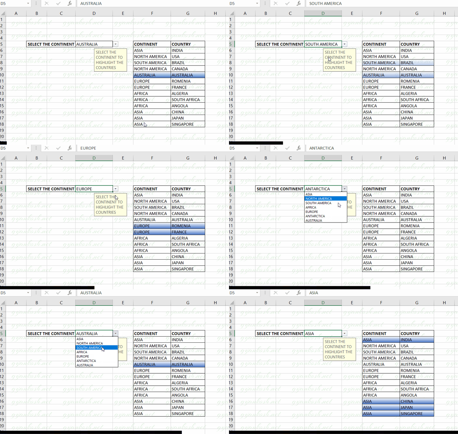
Let us try to create a list where we can highlight the countries lying in a particular continent by selecting the continent from a drop-down list. Something like, one shown in the picture below.

SOLUTION:

This problem comprises different steps for the solution. Here is the list. 

1. Creating a dropdown with continent names as the dropdown options.

2. Setting the CONDITIONAL FORMATTING rule for the given data to highlight the cells containing the countries of the selected continent.

3. Setting the format for the highlighted cells. 

STEP 1:

CREATING A DROPDOWN LIST FOR CONTINENTS LIST

Follow the steps to create a dropdown list.

[ THE COMPLETE DETAILS OF CREATING A DROPDOWN ARE HERE ]

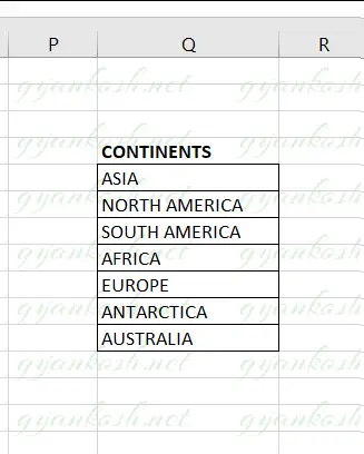
1. Create a simple list of the continents which will be used as the source for the dropdown.
2. The list can be on the same sheet or another sheet as per convenience.

3. Create a LABEL as SELECT THE CONTINENT.
4. Next to the LABEL select the cell, where we’ll populate our dropdown list.
5. Go to DATA TAB > DATA VALIDATION DROPDOWN > DATA VALIDATION

[ THE COMPLETE DETAILS OF CREATING A DROPDOWN ARE HERE ]

6. A dialog box will open as shown below.
7. Select LIST from the ALLOW DROP DOWN as shown in the first picture.
8. After choosing the LIST OPTION, select the source as the range containing the continents. We can directly enter the range or can choose it using the mouse.
9. After choosing the source, we can directly click OK to close the dialog box or we can choose the tab INPUT MESSAGE and choose the INPUT MESSAGE as SELECT THE CONTINENT TO HIGHLIGHT THE COUNTRIES as shown in the last picture.
10. Click OK.

After clicking OK, the dropdown list has been inserted in the cell.

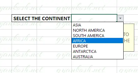
STEP 2: CREATE CONDITIONAL FORMATTING RULES TO HIGHLIGHT THE COUNTRIES OF THE SELECTED CONTINENT

FOLLOW THE STEPS TO ADD CONDITIONAL FORMATTING RULES

1. Select the data excluding the headers.

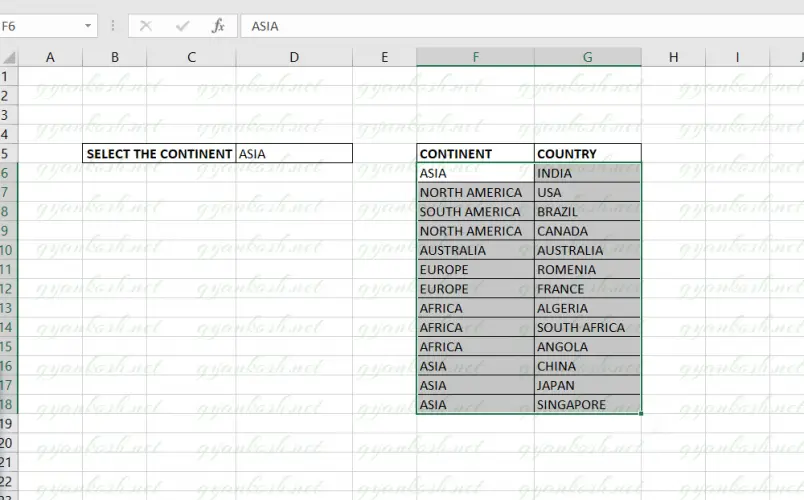
2. Go to HOME TAB > CONDITIONAL FORMATTING DROP DOWN > NEW RULE.

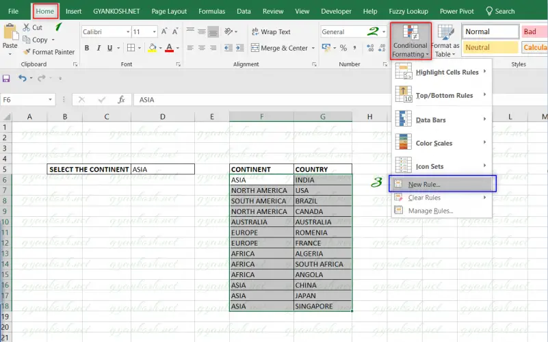
3. As we click the NEW FORMATTING RULE, the dialog box will open.
4. Choose the last option – USE A FORMULA TO DETERMINE WHICH CELLS TO FORMAT.
5. Enter the formula as =$D$5=$F6. [D5 contains our selected continent and F6 is the first cell of the selection. $ has been applied to make the reference absolute for the selection as we don’t want to the selection to go relative whereas the F6, we want the column to be fixed so apply $ before F. [ Learn Conditional Formatting for details ]
6. After entering the formula, click FORMAT BUTTON as shown in the picture below.

7. As we click the format button, a FORMAT CELLS DIALOG BOX opens up.
8. Choose the format as per your choice.
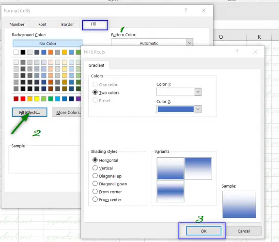
9. We went for FILL TAB > FILL EFFECTS > AND CHOSE AN EFFECT AS SHOWN IN THE PICTURE BELOW.
10. You can choose the format of your own. This format will be visible in all the cells which satisfy the rule we entered.

10. Click OK.
11. We are done.

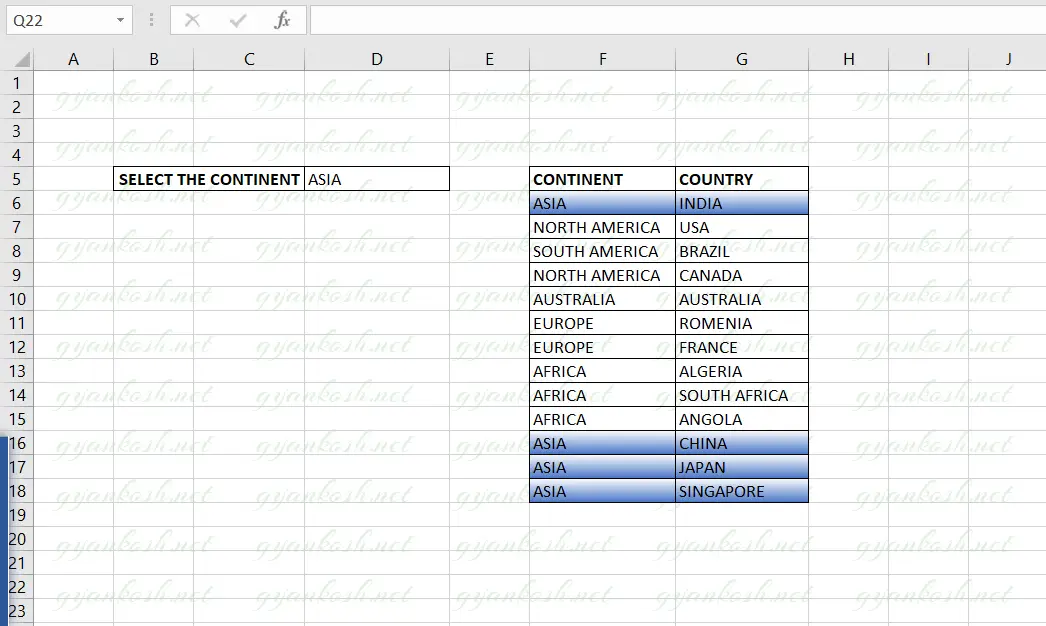
CHECKING THE OUTPUT:

12. We can check the example by selecting the continent from the dropdown.

These were a few usages of conditional formatting based on text in Excel.

SUGGESTED READS:

ONE MORE EXAMPLE FOR CONTROLLING THE CONDITIONAL FORMATTING WITH THE TEXT OR NUMBERS AT OTHER POSITIONS IS HERE.

CREATING A SIMPLE GANTT CHART IN GOOGLE SHEETS

ALTHOUGH, THE ARTICLE SHOWS THE USAGE OF CONDITIONAL FORMATTING IN GOOGLE SHEETS, BUT IT IS COMPLETELY UNDERSTANDABLE AND WORTH READING. TAKE A LOOK AT MORE EXCEL TRICKS. YOU MAY FIND SOMETHING INTERESTING. 

HOW TO HIGHLIGHT THE CURRENT DAY OF THE WEEK USING CONDITIONAL FORMATTING IN EXCEL?

This article shows another useful usage of conditional formatting in Excel.

HOW TO COPY CONDITIONAL FORMATTING IN EXCEL?

The article discussed the copying of conditional formatting in Excel.

HOW TO USE CONDITIONAL FORMATTING BASED ON ANOTHER CELL IN EXCEL?

Control the data based on another cell value.

LEARN DIFFERENT EXCEL TRICKS

THERE’S ALWAYS ROOM FOR IMPROVEMENT.

KINDLY GIVE YOUR VALUABLE SUGGESTIONS.