Table of Contents
- INTRODUCTION
- PREREQUISITES
- APPLYING CONDITIONAL FORMATTING TO FIRST TABLE
- WAY 1 : APPLY THE SAME RULES AGAIN ON THE NEW DATA
- WAY 2 : EDIT THE RANGE OF THE ALREADY APPLIED RULE
- WAY 3 : DIRECT COPY AND PASTE OF CONDITIONAL FORMATTING
INTRODUCTION
Conditional Formatting is one of the frequently used feature of the EXCEL but the most important point about the EXCEL WORKING is that we can never fix the number of ways any problem can be solved in this amazing software.
As we already know
Conditional formatting is the formatting [ font, color, fill color , size etc. ] of data as per its value of the content of the cells.
CLICK HERE TO LEARN ABOUT CONDITIONAL FORMATTING.
It makes our task so easy which you can understand from the following example.
Suppose we have a group of 100 entries and we need to identify the entries between a very small range say 70 to 85. So conditional formatting lets us, set up a rule to highlight such cells with some color to immediately take our notice of those cells. Not just this but we can put a rule for ranges to highlight the cells with different colors. It can be applied to thousands of cells.
Let us take a scenario where we have already applied the conditions to our data.
We have more data on which we need the same conditions and the same rules. What can we do now?
We can apply the same rules again OR we can try to copy the conditional formatting rules from the ALREADY CONDITIONED DATA and paste it fast on the new data to achieve the same results.
It is very obvious that the results from the second option will be fast and efficient . It is going to save a lot of time for us.
So, in this article , we’ll learn the best ways to copy the conditional formatting from one data to another.
PREREQUISITES
IT IS SUPPOSED THAT YOU KNOW THE BASICS OF APPLYING CONDITIONAL FORMATTING AND UNDERSTAND IT WELL.
IF NOT,
DIFFERENT WAYS TO COPY CONDITIONAL FORMATTING IN EXCEL
There are a few ways which can be used to copy the conditional formatting in excel easily.
- Applying the CONDITIONAL FORMATTING to the NEW DATA in the standard way.
- Editing the range of Formula of the already applied data.
- Direct Copy- Paste option of the Conditional formatting.
We’ll discuss all the three ways [ Except S.No. 1 as there is a separate article for that ] with an example for better understanding.
EXAMPLE: COPY CONDITIONAL FORMATTING IN EXCEL
Its always easy to learn through the example.
Let us take an example and copy its conditional formatting to a new data set.
EXAMPLE DETAILS:
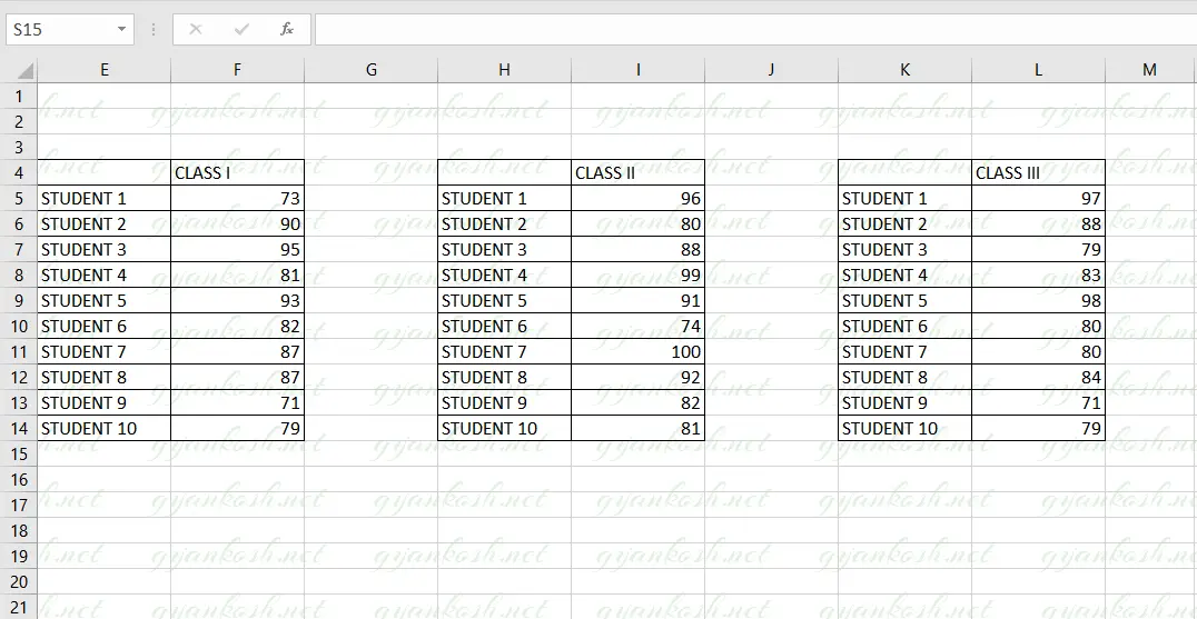
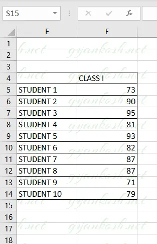
Let us take an example with the marks of 10 students of class A.
We want to highlight the students with marks more than 90.
We already have this formula applied to one data of Class I. We want to copy the formatting and apply it on Class II and class III.
| CLASS I | |
| STUDENT 1 | 73 |
| STUDENT 2 | 90 |
| STUDENT 3 | 95 |
| STUDENT 4 | 81 |
| STUDENT 5 | 93 |
| STUDENT 6 | 82 |
| STUDENT 7 | 87 |
| STUDENT 8 | 87 |
| STUDENT 9 | 71 |
| STUDENT 10 | 79 |
| CLASS II | |
| STUDENT 1 | 96 |
| STUDENT 2 | 80 |
| STUDENT 3 | 88 |
| STUDENT 4 | 99 |
| STUDENT 5 | 91 |
| STUDENT 6 | 74 |
| STUDENT 7 | 100 |
| STUDENT 8 | 92 |
| STUDENT 9 | 82 |
| STUDENT 10 | 81 |
| CLASS III | |
| STUDENT 1 | 97 |
| STUDENT 2 | 88 |
| STUDENT 3 | 79 |
| STUDENT 4 | 83 |
| STUDENT 5 | 98 |
| STUDENT 6 | 80 |
| STUDENT 7 | 80 |
| STUDENT 8 | 84 |
| STUDENT 9 | 71 |
| STUDENT 10 | 79 |
APPLYING CONDITIONAL FORMATTING TO FIRST TABLE
As we already discussed, conditional formatting will be applied to class I. We’ll discuss the procedure briefly as it is discussed in detail in a separate article. Link is given below.
CLICK HERE FOR COMPLETE DETAILS ABOUT CONDITIONAL FORMATTING.
FOLLOW THE STEPS TO CONDITIONAL FORMAT AND HIGHLIGHT THE MARKS MORE THAN 90 MARKS IN CLASS I.
- Go to HOME TAB and click CONDITIONAL FORMATTING > HIGHLIGHT CELL RULES >GREATER THAN.
- GREATER THAN dialog box will open.
Look at the picture below.
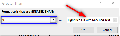
- Enter the value as 90 and choose the formatting. Current selection is LIGHT RED FILL WITH DARK RED TEXT. Other options can be chosen from the drop down.
- Click OK.
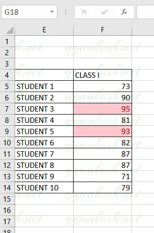
- The result will be like this.
WAY 1 : APPLY THE SAME RULES AGAIN ON THE NEW DATA
The first way to copy the conditional formatting is to look for the formula used and apply the same rule to the new data in the exactly same way as we did in the previous section above.
WAY 2 : EDIT THE RANGE OF THE ALREADY APPLIED RULE
PRE-PLANNING
We intend to change the range of the already applied rule.
It means that we’ll edit the already applied formatting rules [ on CLASS I] and edit the cells on which it is applied, which will directly apply the same rule to the new range also.
STEPS TO COPY THE CONDITIONAL FORMATTING
- Select any cell of the class I marks where we have already applied the conditional formatting.
- Go to HOME TAB > CONDITIONAL FORMATTING > MANAGE RULES.
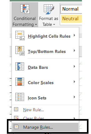
- As we click MANAGE RULES, the RULE MANAGER DIALOG BOX will open.
- This dialog box contains all the formatting rules applied, range and much information about the conditional formatting.
- The following picture shows the CONDITIONAL FORMATTING RULE MANAGER.
- The blue rectangle marks the APPLIES TO field which contains the cell address where the RULE IS APPLIED.
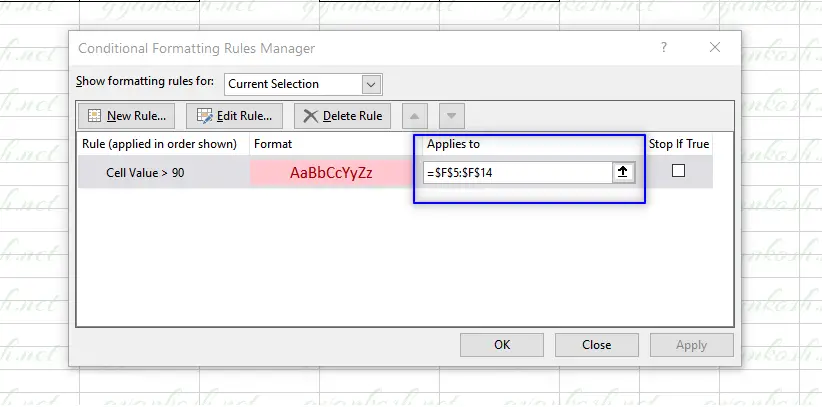
Now, we can see the APPLIES TO field contains the field address where the rule is applied which we want to copy.
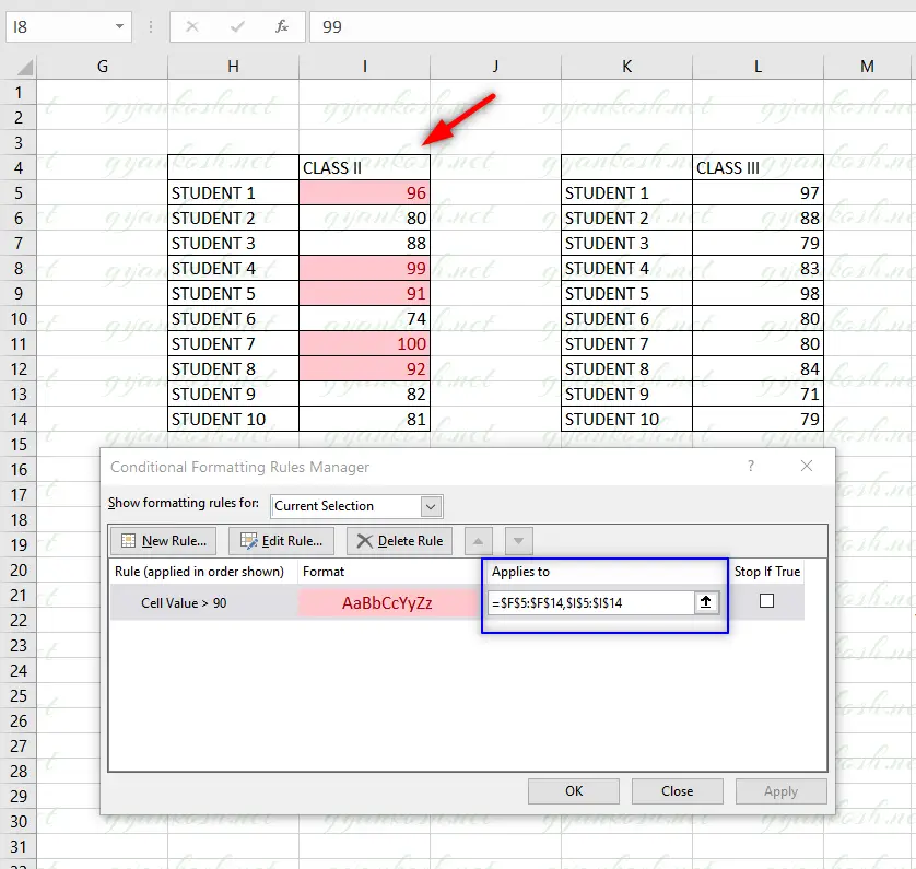
- Simply put a comma and add the additional range with this.
- Put in APPLIES TO FIELD ,$I$5:$I$14.
- Click OK.
- The conditional formatting is copied from the CLASS I to CLASS II.
WAY 3 : DIRECT COPY AND PASTE OF CONDITIONAL FORMATTING
PRE-PLANNING
There is a simple option given in PASTE SPECIAL to paste the formatting.We’ll copy the conditional formatting [ simple copy ] and special paste it on the new data. [ CLASS III ]
STEPS TO COPY THE CONDITIONAL FORMATTING
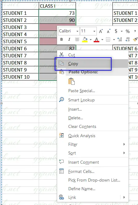
- Select any cell of the class I marks where we have already applied the conditional formatting. [ We can choose one cell or a group of cells ]
- Right Click and choose COPY. [ Simple Copy ]
After we have copied any cell or cells , select all the cells where we want to paste the formatting.
For our example, as we want to paste the formatting on CLASS III, we’ll select the cells from L4 to L14.
- Right Click > Paste Special and choose FORMATS.
- The CONDITIONAL FORMATTING RULES of the copied cells will be applied to the CLASS III also.
In this way we can copy conditional formatting from one text area to other.