Table of Contents
- INTRODUCTION
- WHY DO WE NEED HIGHLIGHTING THE DAY OF A WEEK?
- CONCEPT BEHIND HIGHLIGHTING THE CURRENT DAY OF THE WEEK
- CREATING THE AUTOMATICALLY HIGHLIGHTING DAY OF THE WEEK IN EXCEL
- STEP 1: PREPARE THE DATA
- STEP 2: APPLY CONDITIONAL FORMATTING
INTRODUCTION
CONDITIONAL FORMATTING is a great option to highlight any important values in Excel.
Conditional formatting is the formatting [ font, color, fill color , size etc. ] of data as per its value of the content of the cells based on the given condition.
Conditional formatting is simply a FORMATTING OF THE DATA ON THE BASIS OF ITS VALUES which highlights the data of our use or the data which satisfies the condition.
Conditional Formatting is a frequent requirement in small or big reports which makes it mandatory for everybody to learn if you are using GOOGLE SHEETS , EXCEL or any other spreadsheet application.
In this article, we’ll learn yet another simple technique of highlighting the current day in Excel using conditional formatting.
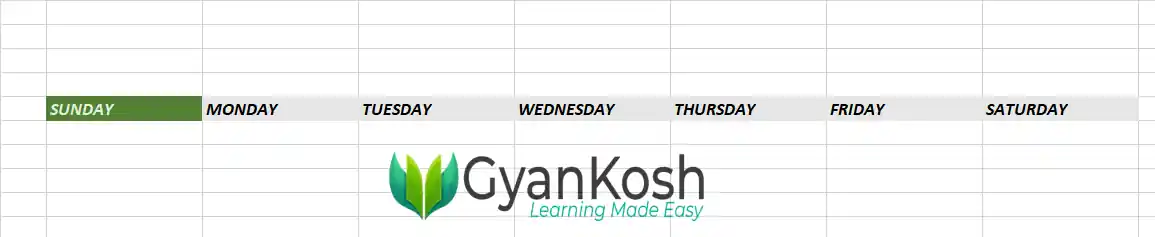
We’ll be creating something like this.

WHY DO WE NEED HIGHLIGHTING THE DAY OF A WEEK?
This utility can be a part of any live or shared Excel sheet where you ‘ll be maintaining the daily data.
All the days are present and the current day will be highlighted.
This can also be a part of the calendar to highlight the current day.
There can be many other situation where we can make use of this.
CONCEPT BEHIND HIGHLIGHTING THE CURRENT DAY OF THE WEEK
The concept is very simple.
We’ll enter all the Days of the Week.
We’ll get the current day and compare it to the given days.
Once the comparison is successful,, we’ll format the day and highlight it.
Let us find out the steps to create the desired current day highlighter.
We’ll be making the use of CONDITIONAL FORMATTING AND TEXT FUNCTION in this article. You can learn the both here.
CREATING THE AUTOMATICALLY HIGHLIGHTING DAY OF THE WEEK IN EXCEL
Let us start the process.
We’ll do it in two steps.
- Preparing the data.
- Applying the formatting.
STEP 1: PREPARE THE DATA
Let us prepare the data first.
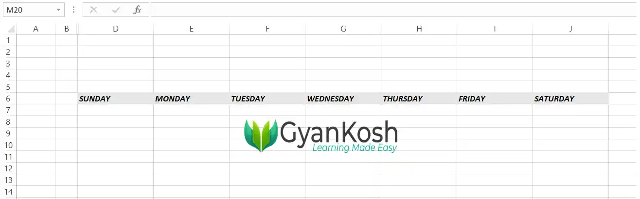
Type all the names of SEVEN DAYS of a week horizontally or vertically as per your requirement. Each name in different cells.
We have used them horizontally for the example discussed.
Give them any formatting , fonts, fill color, font color etc. as per your requirement.
We have used bold, italics and given them a little light grey color.
The picture below shows the picture.
*NO ISSUES WHEREVER YOU PUT THE WEEKDAYS IN THE SHEET. WE HAVE NOTHING TO DO WITH THE CELL ADDRESSES/REFERENCES.
After the data is prepared, it is time to put the conditional formatting on this data.
STEP 2: APPLY CONDITIONAL FORMATTING
After the data is ready, we can go for applying the conditional formatting.
FOLLOW THE STEPS TO USE CONDITIONAL FORMATTING TO HIGHLIGHT THE CURRENT DAY:
- Select the data.
- Our example data lies between D6:J6, so we selected the same.
- After selecting the data , go to the CONDITIONAL FORMATTING [ under the HOME TAB ] , click the drop down and choose NEW RULE as shown in the picture below.
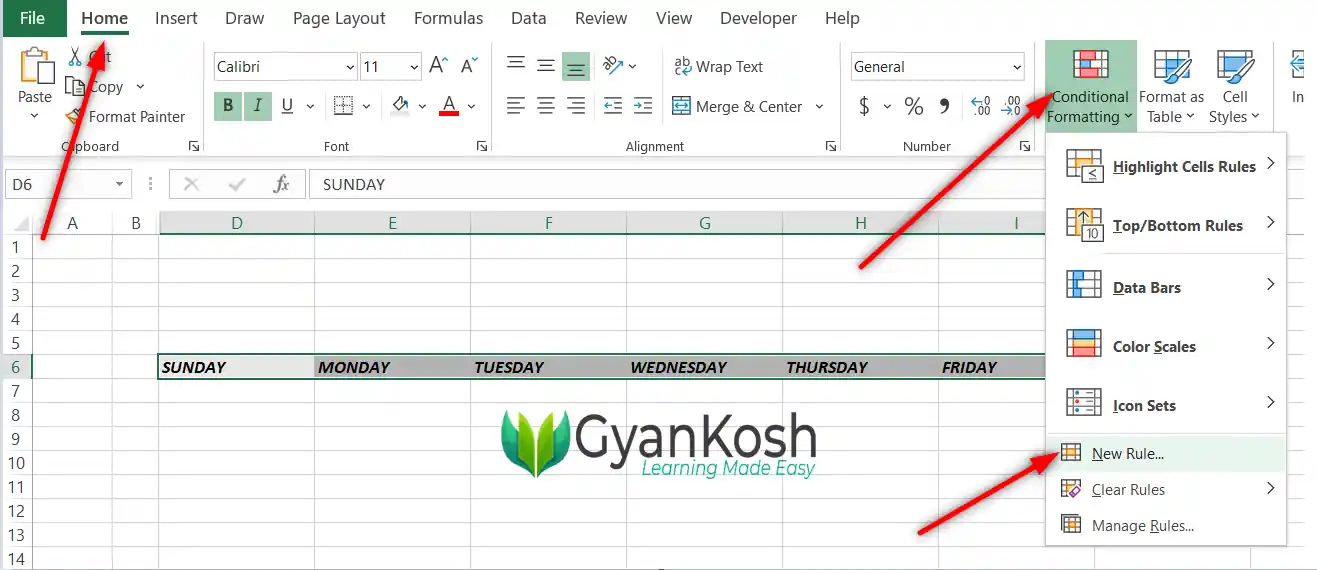
- As we click NEW RULE, a dialog box will open.
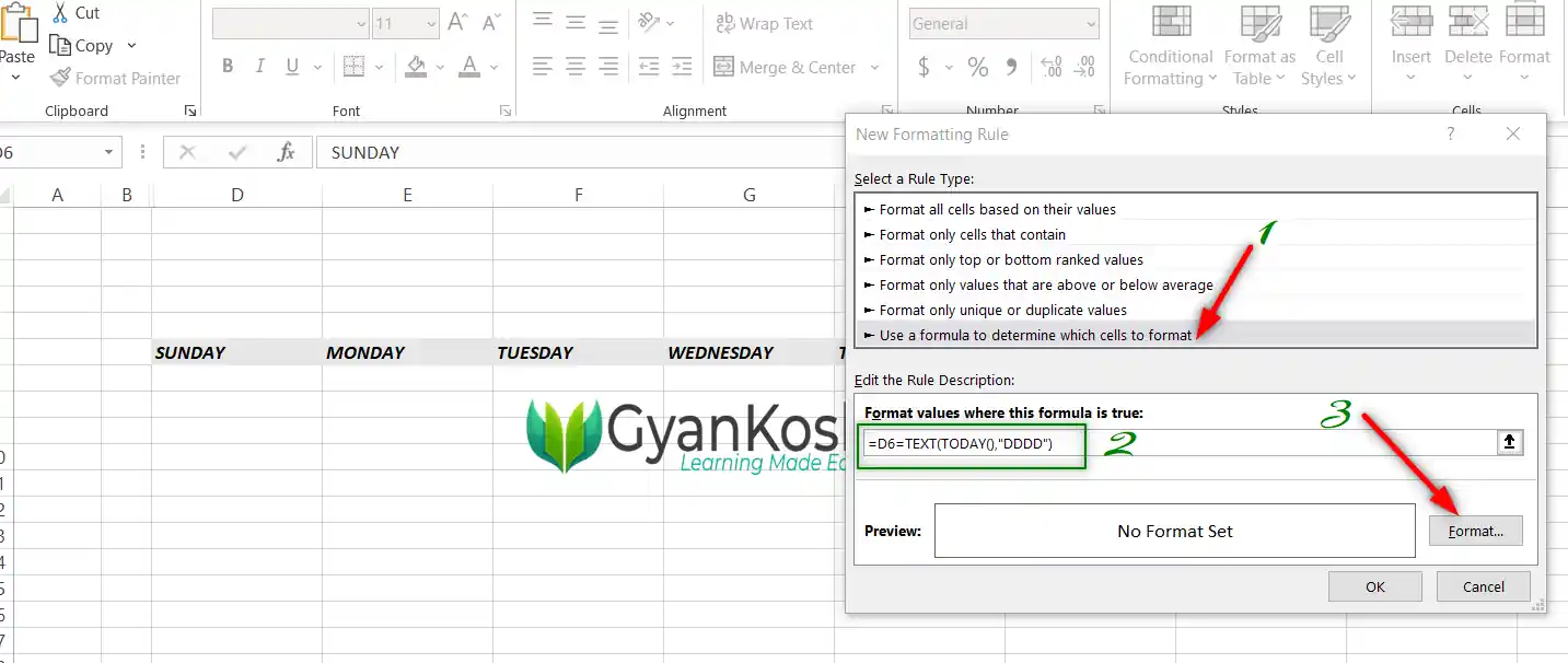
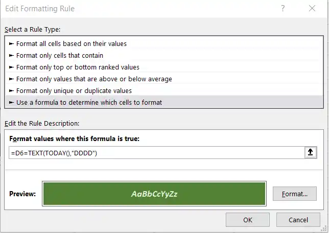
- Choose USE A FORMULA TO DETERMINE WHICH CELLS TO FORMAT denoted by 1 in the picture below.
- As we choose 1, a space for the formula will appear.
- Enter the formula as =FIRST CELL OF THE SELECTION=(TEXT(TODAY(),”DDDD”)
- As our example’s selection’s first cell is D6, our formula becomes =D6=TEXT(TODAY(),”DDDD”).
- Don’t click OK, but go to FORMAT.
- Format option, opens the FORMAT CELLS dialog box.
THIS IS THE FORMAT WHICH IS GIVEN TO THE CELL FULFILLING THE CONDITIONS I.E. OUR RESULT.
- We simply chose a fill color to be green and FONT COLOR to be white.
- After all the format is set , click OK.

After everything is done, we’ll be back in the first screen , but the result will be showing the format of the resulting cells.
You can see in the picture below that sample result is in the green with a white font color.
- After checking the output format, click OK.
- We are done.
- The result is shown below.