Table of Contents
- INTRODUCTION
- BUTTON LOCATION: CONDITIONAL FORMATTING
- STEPS TO START CONDITIONAL FORMATTING:
- CONDITIONAL FORMATTING :DIFFERENT AVAILABLE OPTIONS
- CONDITIONAL FORMATTING: NEW RULE[custom]
INTRODUCTION
In this article, we’ll discuss the ways to do conditional formatting in Excel.
To have the knowledge of Conditional formatting is very important if we want to apply Excel in our day to day jobs.
Conditional formatting is the formatting [ font, color, fill color , size etc. ] of data as per its value of the content of the cells.
It is one of the most versatile functions present in Excel and very easy to apply and learn.
It makes our task so easy which you can understand from the following example.
Suppose we have a group of 100 entries and we need to identify the entries between a very small range say 70 to 85. So conditional formatting lets us, set up a rule to highlight such cells with some color to immediately take our notice of those cells. Not just this but we can put a rule for ranges to highlight the cells with different colors. It can be applied to thousands of cells.
Let us lean the way to apply conditional formatting to our data.
BUTTON LOCATION: CONDITIONAL FORMATTING
STEPS:
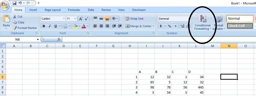
- Go to the HOME TAB( Conditional formatting option is present under HOME TAB).
- Conditional button can be found on the “HOME TAB” under STYLES SECTION. The location is marked in the following picture.
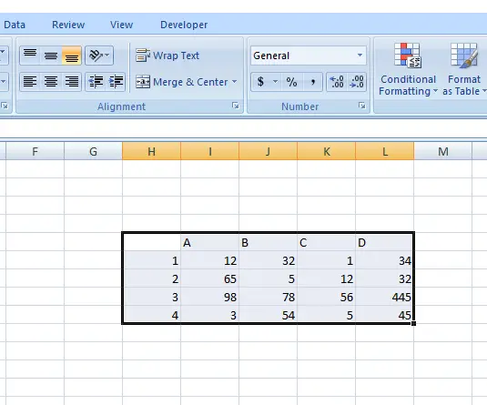
EXAMPLE 1: DATA SAMPLE
The following picture shows the sample data we will be using in the example.
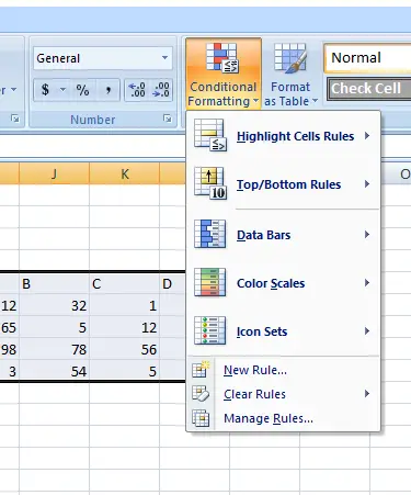
STEPS TO START CONDITIONAL FORMATTING:
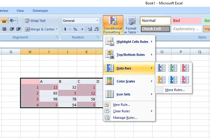
- CLICK on CONDITIONAL FORMATTING BUTTON. The following menu will open.
CONDITIONAL FORMATTING :DIFFERENT AVAILABLE OPTIONS
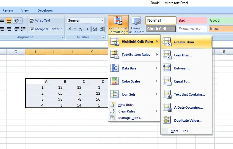
HIGHLIGHT CELL RULES
Select the data and choose any action under highlight cell rules and it’ll highlight(COLOR THE CELLS TO MAKE THEM DIFFERENT FROM OTHER CELLS) those particular cells where the value satisfies your given condition.
FOR THE EXAMPLE Lets choose ” LESS THAN” formatting and see the result. Put the value as “30”in the dialog box.
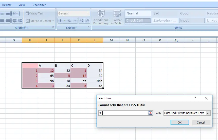
In this example, we can see that we want the values which are LESS THAN 30. So it highlighted the values which are less than 30 with a color.
In this DEMO, we can see that we want the values which are LESS THAN 30. So Excel highlighted the values which are less than 30 with a color.
Similarly we can choose any formatting from the menu. All the names given are self explanatory easy to use. Just put the value in the dialog box and click ok, Excel will do it for you.
Some other available options are given below.
ADDITIONAL HIGHLIGHT CELL RULES
In addition to the above rule of LESS THAN, there are many other options available. Let us have a look at them.
GREATER THAN-Highlighting all the numbers greater than a particular value.
LESS THAN– Highlighting all the number less than a particular value.
BETWEEN– Highlighting all the numbers between two particular values.
EQUAL TO-Highliting all the numbers equal to a given value.
TEXT THAT CONTAINS– Highlighting the cells which contain the user given letter sequence.
A DATE OCCURRING – Highlighting the cells which contain the date as per the selected conditions like yesterday, last 7 days, coming 7 days etc.
DUPLICATE VALUES– Highlights all the repeated values.
TOP BOTTOM RULES
The next options after the highlighting rules is the TOP/BOTTOM rules.
These rules contains READY TO USE functions for TOP OR BOTTOM VALUES. A brief description is given below.
- TOP 10 ITEMS-Highlight top 10 values of the data.
- TOP 10 %- Highlight top 10% values of the data.
- BOTTOM 10 ITEMS-Highlight bottom 10 values of the data.
- BOTTOM 10 %-Highlight bottom 10% values of the data.
- ABOVE AVERAGE-Highlight the values which are above the average of the data.
- BELOW AVERAGE-Highlight the values which are below the average of the data.
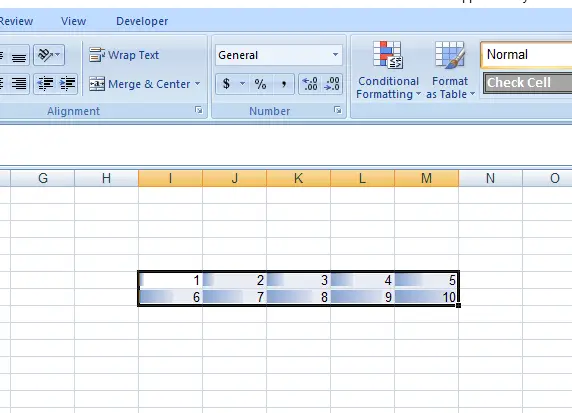
CONDITIONAL FORMATTING:DATA BARS
It shows the bars in each cell as per the value in the cell(More the value, more filled is the bar) .
The way of using the bars is also the same as that of the highlighting the cell rules. Same is with the color scales. Color scales chooses the color for a particular range.
The following picture shows the use of DATA BARS. More the value, more filled is the cell.
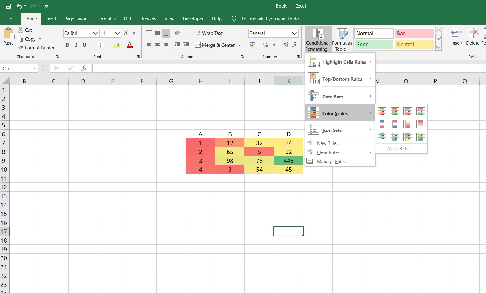
CONDITIONAL FORMATTING:COLOR SCALES
Like the data bars, we have color scales option also which shows different colors for different values. e.g. green for higher values and red for lower whereas yellow for the middle.
CONDITIONAL FORMATTING: NEW RULE[custom]
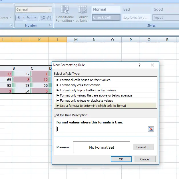
New rule is the option given for you to make any custom rule (Self Defined) ,if you want.
Some already listed options are also shown in NEW RULE dialog box .
Let us see what we can do with Custom Rule of conditional formatting.
In this option, you can use the various formatting options as per your choice. The answer will appear in a format as per your definition set through the FORMAT button in the lower right corner.
Let us give it a try.
Suppose we want that any cell with value more than 65 should be highlighted.
For this, we need to put formula for one cell (first cell at the left upper corner) as rest of the formula will be relative.
CONDITIONAL FORMATTING: NEW RULE EXAMPLE 1
We will highlight those numbers whose values are greater than 65.
For that, as per the example , we’ll put formula for the Cell H6 and then extend it to others. The formula used in this section should always return “true or false” only.
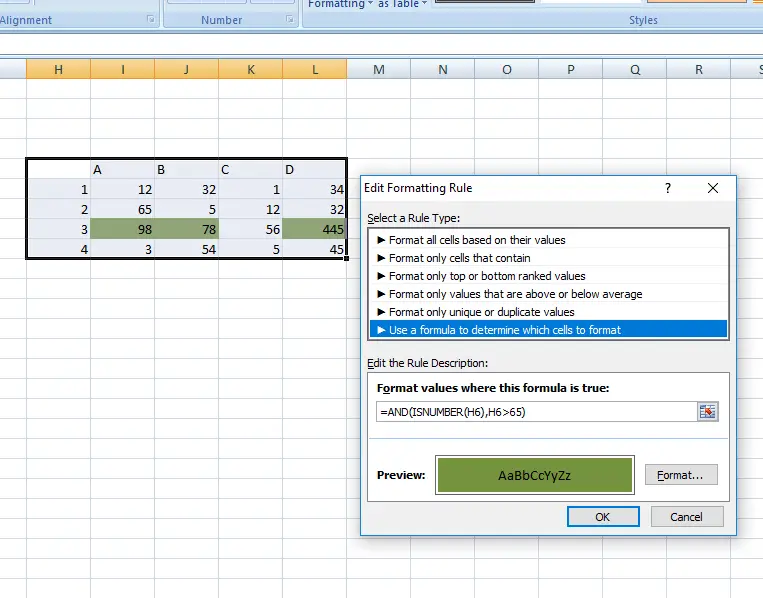
- Select the range or all the cells on which the conditions is to be applied. Now click CONDITIONAL FORMATTING BUTTON> NEW RULE.
- Put the formula as “=condition for the first cell”. Choose the format as I have chosen a fill color for highlighting. Please mind that formula must start with “=”.
In this formula we are putting a AND statement and its checking whether h6 is number and whether h6>65. Both will be multiplied as (AND function multiplies the values) return true or false). - Now change the format as you want the output.
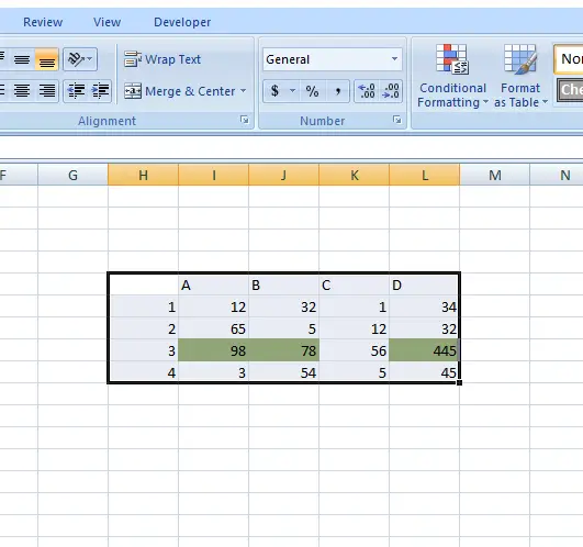
- Click OK.
The cells fulfilling the conditions will be highlighted.
USER DEFINED FORMULA :EXAMPLE 2
Let us try one more example of Custom Formula or User defined formula for better understanding.
We’ll find out a mid range from given data.
Suppose we have a data of maximum temperatures of any city. We’ll find out the days, on which the temperature was within a certain range.
| TEMPERATURE OF CITY A (15 DAYS) | |
| DAY | TEMPERATURE (°C) |
| 1 | 25 |
| 2 | 28 |
| 3 | 29 |
| 4 | 32 |
| 5 | 28 |
| 6 | 30 |
| 7 | 33 |
| 8 | 35 |
| 9 | 37 |
| 10 | 34 |
| 11 | 33 |
| 12 | 32 |
| 13 | 30 |
| 14 | 31 |
| 15 | 30 |
We will find out the temperatures greater than 30 upto 40 degree celcius. So let us try to apply custom formula for formatting on this table. Look at the following picture.
We select the cells where we want to apply the conditions.
Go to the New formula option.
Put the formula as
=AND(J6>30,J6<=40)
which will return a true for the cells where temperature is greater than 30 and upto 40.
The format can be chosen as per choice. Any color or font can be set.
Press Enter
and we have the excel highlight the cells which fulfill our conditions.