Table of Contents
- INTRODUCTION
- WHERE DO YOU FIND CONDITIONAL FORMATTING OPTION IN GOOGLE SHEETS ?
- STEPS TO STRIKETHROUGH NUMBERS LESS THAN 100 USING CONDITIONAL FORMATTING
- EXAMPLE 2: REMOVE STRIKETHROUGH USING CONDITIONAL FORMATTING FROM THE CELLS IN GOOGLE SHEETS
INTRODUCTION
In this article, we’ll learn the way to strikethrough in Google Sheets using the concept of conditional formatting.
Conditional formatting is the formatting [ font, color, fill color , size etc. ] of data as per its value of the content of the cells.
It is one of the most versatile functions present in GOOGLE SHEETS and very easy to apply and learn.
It makes our task so easy which you can understand from the following example.
Suppose we have a group of 100 entries and we need to identify the entries between a very small range say 70 to 85. So conditional formatting lets us, set up a rule to highlight such cells with some color to immediately take our notice of those cells. Not just this but we can put a rule for ranges to highlight the cells with different colors. It can be applied to thousands of cells.
WHERE DO YOU FIND CONDITIONAL FORMATTING OPTION IN GOOGLE SHEETS ?
CONDITIONAL FORMATTING OPTION can be found under the INSERT TAB.
Steps to choose conditional formatting option.
- Go to the INSERT MENU.
- Choose CONDITIONAL FORMATTING.
- The options will appear on the right side of the screen.

Let us now learn the way to strikethrough in Google Sheets using conditional formatting. It’ll become more clear using the following examples.
EXAMPLE 1: STRIKETHROUGH THE NUMBERS LESS THAN 100 USING CONDITIONAL FORMATTING
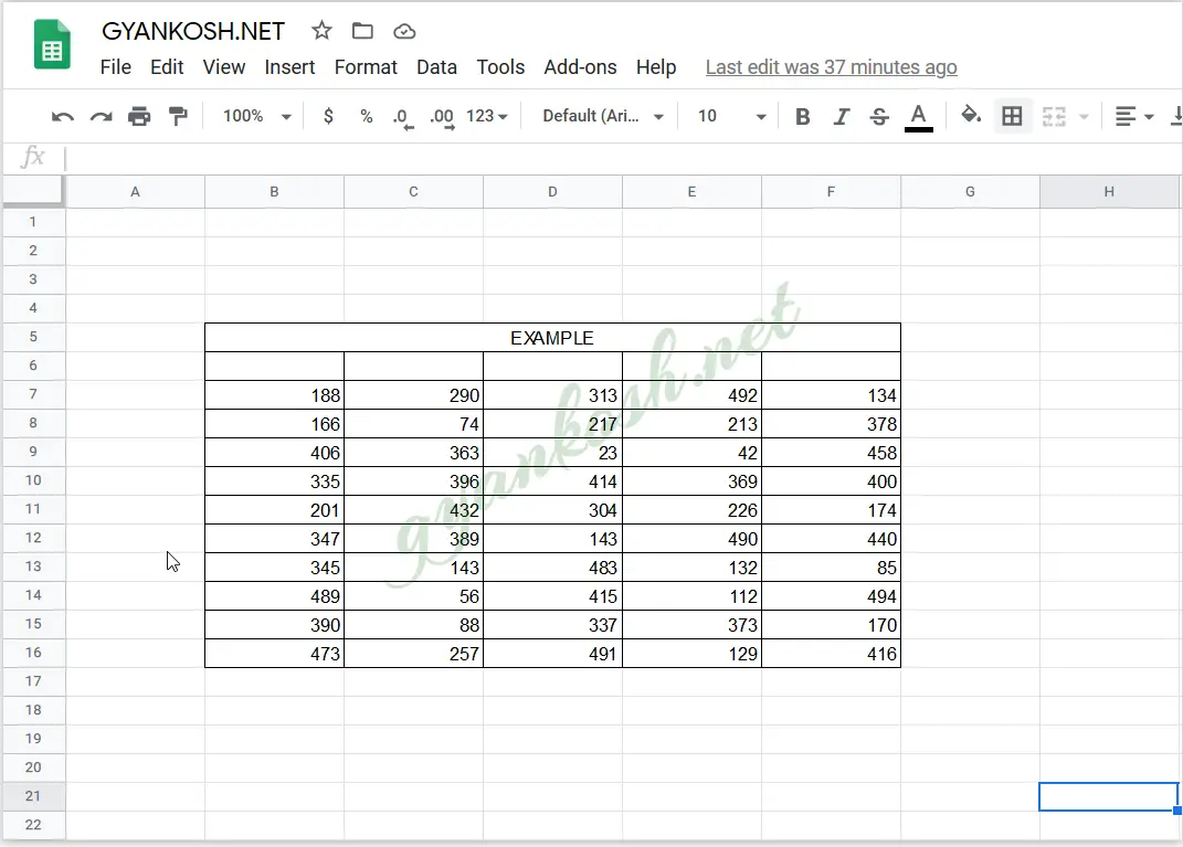
The following picture shows the sample data we will be using in the example. Let us learn conditional formatting using a simple example.
We have data with different numbers . Let us highlight the numbers less than 100.
STRIKETHROUGH IN GOOGLE SHEETS THE NUMBERS LESS THAN 100 IN THE GIVEN DATA
The data used is shown below.
STEPS TO STRIKETHROUGH NUMBERS LESS THAN 100 USING CONDITIONAL FORMATTING
STEPS TO APPLY CONDITIONAL FORMATTING:
- Select the data. [ONLY THE CELLS WITH THE DATA ON WHICH WE WANT TO APPLY CONDITIONS].
- Go to FORMAT MENU> CONDITIONAL FORMATTING.
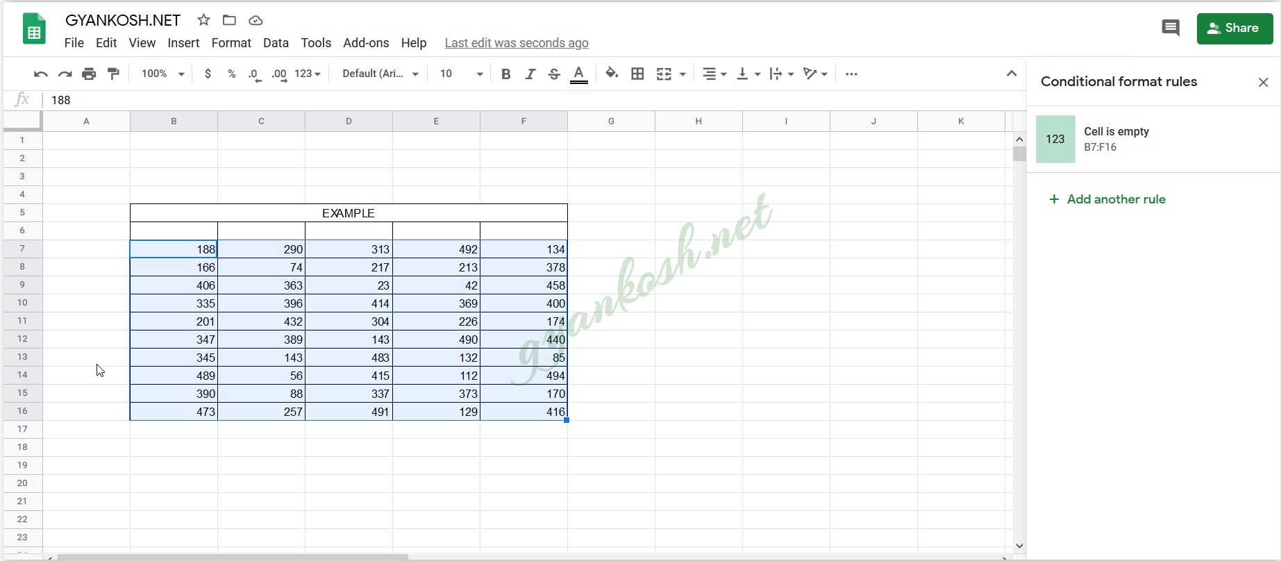
- After clicking the CONDITIONAL FORMATTING OPTION, The screen will be like the one shown above.
- On the right side ,it is the conditional formatting options.
- CLICK THE CONDITIONAL FORMATTING RULES on the right which shows the Range of the selected cells.
- As soon as we click it, CONDITIONAL FORMATTING RULES box will open on the right.
HIGHLIGHT CELL RULES
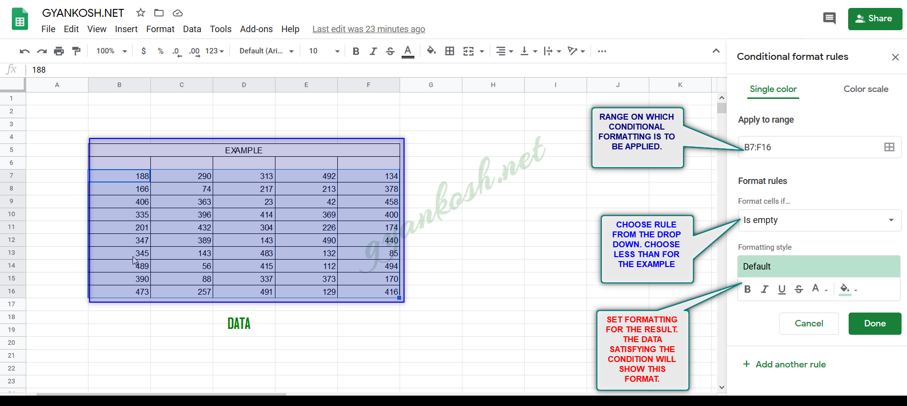
In the CONDITIONAL FORMAT RULES , we have following options.
- APPLY TO RANGE: Put the range on which we want to apply the conditional formatting rules.
- FORMAT RULES: Choose LESS THAN from the given list of rules.
- FORMATTING STYLE: Choose font, font color etc. formatting for the data which will satisfy the values.
All these are shown in the picture below.
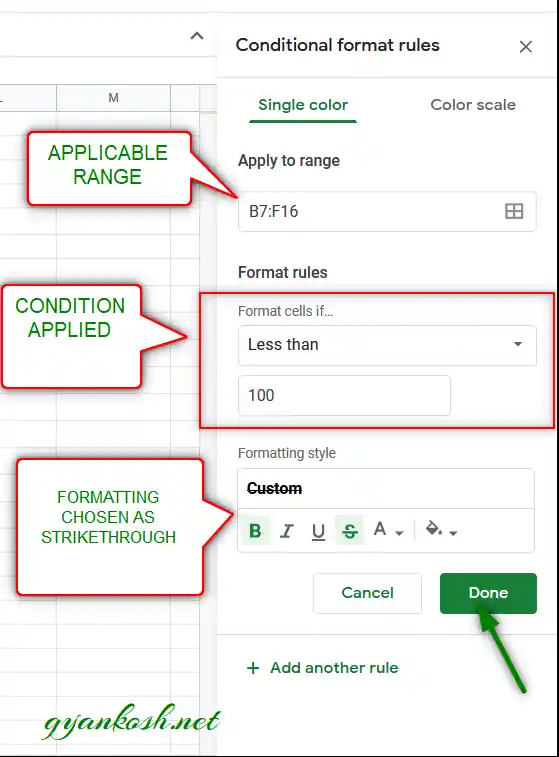
When we choose the Format Rules as LESS THAN, a new field opens up to enter the value LESSER THAN WHICH , all the values will be highlighted.
- Enter 100 in this field as per the requirement.
- Go to Formatting STYLE.
- Choose format of your choice. For our example, we’ll choose STRIKETHROUGH.
- Click OK.
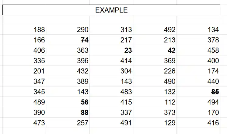
After CLICKING THE DONE button, All the numbers less than 100 are strikethrough or cross out.
The final table is shown below.
This was a simple example of STRIKETHROUGH IN GOOGLE SHEETS USING CONDITIONAL FORMATTING.
EXAMPLE 2: REMOVE STRIKETHROUGH USING CONDITIONAL FORMATTING FROM THE CELLS IN GOOGLE SHEETS
Sometimes, we might need to remove all types of conditional formatting from our sheet.
It can be done using the following steps.
- Select all the cells in which we want to remove the conditional formatting.
- Go to FORMAT MENU and choose REMOVE CONDITIONAL FORMATTING.
- All the STRIKETHROUGH conditional formatting will be removed i.e. All the cells containing the strikethough data will be removed.