Table of Contents
- INTRODUCTION
- PREREQUISITES TO USE SLICER IN EXCEL
- BUTTON LOCATION FOR SLICER
- STEPS TO CREATE A SLICER IN EXCEL
- UNDERSTAND THE STRUCTURE OF SLICER
- STEPS TO USE A SLICER IN EXCEL
- EXPLANATION
INTRODUCTION
Filtering is one of the major operation which is going to be used over and again in our day to day work.
We have got FILTER FUNCTION , a separate filter functionality which we apply on the data already. In addition to this we got a new functionality called SLICERS.
SLICERS are a new way of filtering data in Excel.
Its mostly graphical, easy to use and help us to see what is the current condition of the filtration state.
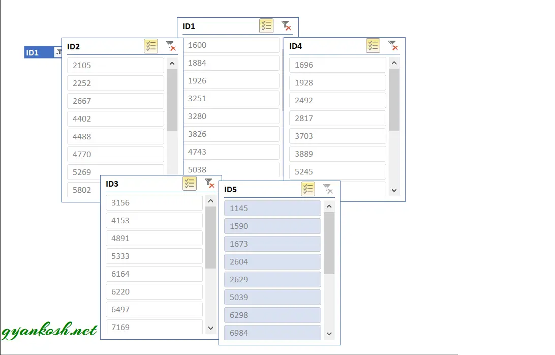
Slicers gives us the option of slicing the columns into small tables which further gives us the control of filtering the data.
The slices are something like this as shown in the picture below.
PREREQUISITES TO USE SLICER IN EXCEL
The SLICER can’t be used anywhere we want.
SLICER is specifically meant for tables only. The table can be a SIMPLE TABLE or the PIVOT TABLE.
Here we’ll be discussing slicer with the help of normal tables only. Slicer for the PIVOT TABLE will be dealt in the PIVOT TABLE article only. So let us try to create a slicer for the table.
BUTTON LOCATION FOR SLICER
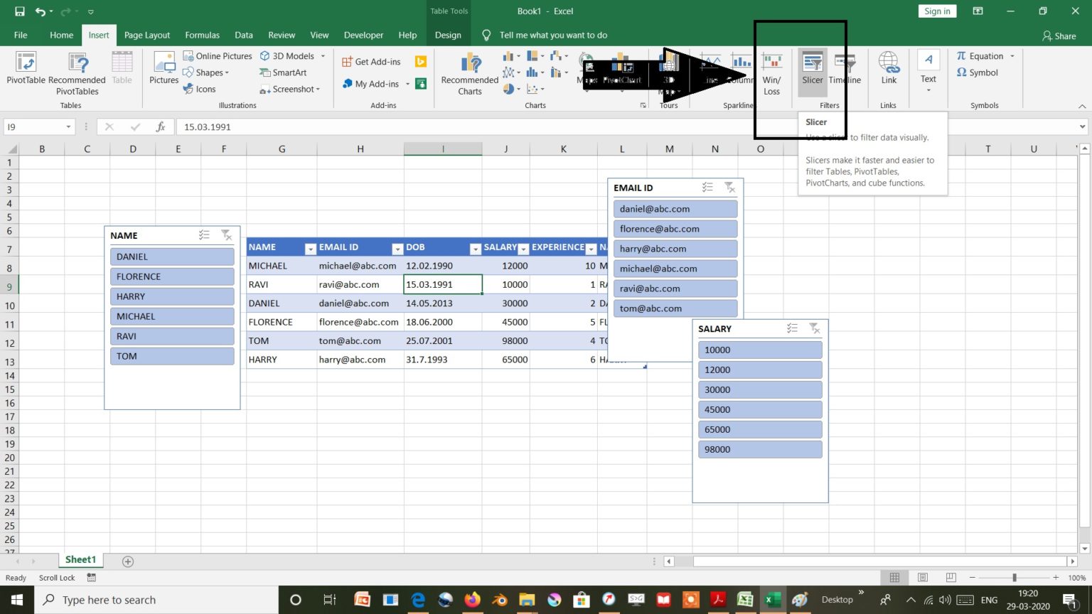
The SLICER is located under the INSERT TAB in FILTER OPTIONS. The picture below shows the button location for SLICER.
STEPS TO CREATE A SLICER IN EXCEL
STEPS:
- Create a table having some data so that we try our slicer on that.
- If you don’t know how to create a table. Click here.
- Click any where in the table.
- Go to INSERT TAB>FILTER OPTIONS and CLICK SLICER.
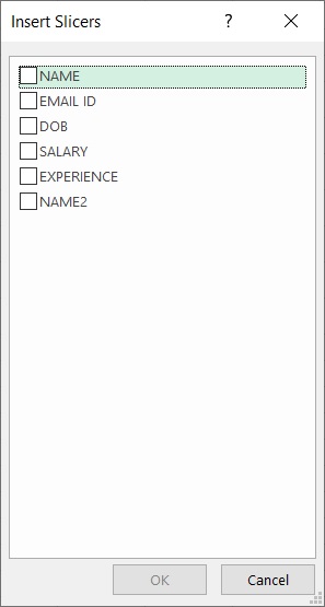
- A small window will open which will list all the headers (column names or row names) to be selected from. We’ll select the options which we want to slice. i.e. which we want to choose from. The following picture shows the options window.
- Select any number of columns from this window and check the boxes to select.
- That many number of slices will be made.
- In our case, we’ll use SALARY and EXPERIENCE, two options.
NOTE: Choose those options which are the basis of filtering. Don’t choose all the options as it’ll only mess up the screen.
AFTER CHOOSING THE OPTIONS, FOLLOWING PICTURE SITUATION WILL APPEAR.
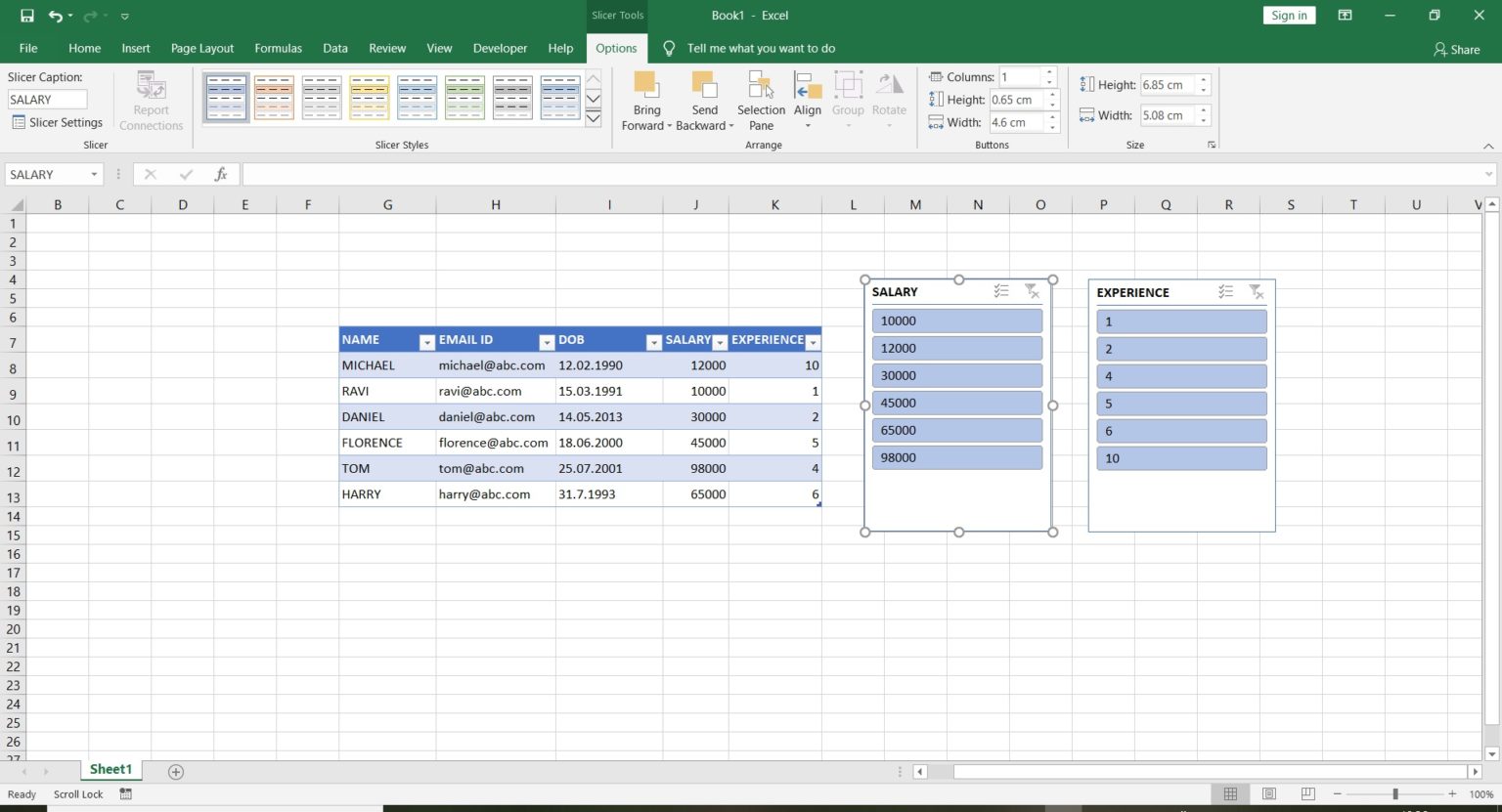
The slicers have been deployed. Now we’ll see how to use them.
UNDERSTAND THE STRUCTURE OF SLICER
The following picture shows the structure of a slicer.
ALL THE BLUE SELECTED LINES IN BOTH THE SLICERS ARE THE CONDITIONS SELECTED.
We can click on the rows of the slicer to check or uncheck them. As a result of this, the table will alter real time.
The two slicers are the two conditions. The result is the table which would alter as per the applicability of the conditions.
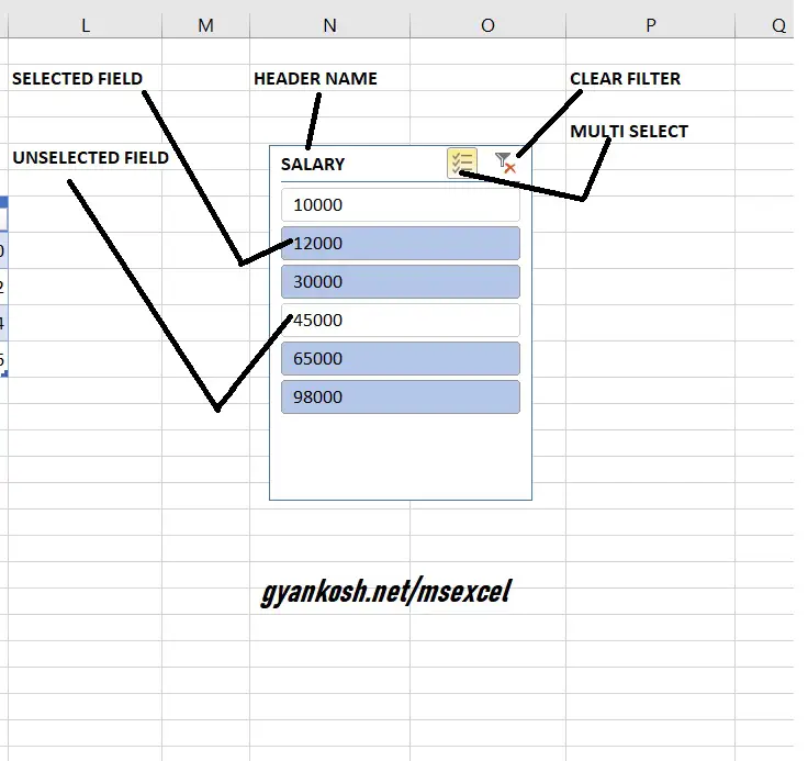
AS PER THE ABOVE PICTURE,
We can see that the heading or category is shown at the top as SALARY.We can click on the field to select it and click again to deselect it.A button in right up corner will clear all the filter.A button to select multi values is also present in the right upper corner.
STEPS TO USE A SLICER IN EXCEL
PLACE BOTH THE SLICER WINDOWS SIDE BY SIDE .
SELECT ANY CONDITION AND THE TABLE WILL CHANGE THE FORM IN THE SAME TIME.TABLE WILL SHOW THE FIELDS WHICH FULFILL THE SELECTED CONDITIONS.
THE FOLLOWING PICTURE SHOWS THE RESULT.WE’LL FIND THE FOLLOWING CONDITIONS.BOTH THE SLICERS ARE DESELECTED
1. SALARY UPTO 30000.
2. SALARY MORE THAN 30000 AND EXPERIENCE LESS THAN 7 YEARS.
3. SALARY BETWEEN 35K TO 60K AND EXPERIENCE BETWEEN 3 TO 10 YEARS.
EXPLANATION
JUST HAVE A LOOK AT THE ANIMATION PICTURE ABOVE.
We fulfilled all the three conditions by just selecting and deselecting the slicers.
Both the conditions are matched and result is kept in the result table.
This is how easy it is.