Table of Contents
- INTRODUCTION
- WHAT IS A PIVOT TABLE IN GOOGLE SHEETS ?
- WHERE TO FIND THE PIVOT TABLE BUTTON LOCATION IN EXCEL?
- BENEFITS OF USING PIVOT TABLES IN EXCEL
- STEPS TO CREATE PIVOT TABLE IN EXCEL
- UNDERSTAND DIFFERENT OPTIONS AND SCREENS WHILE CREATING A PIVOT TABLE
- PIVOT TABLE SHEET DESCRIPTION IN EXCEL
- CHANGE THE CALCULATION FORMULA IN PIVOT TABLE IN EXCEL
INTRODUCTION
PIVOT TABLE is a well known feature of EXCEL which everybody of us might have heard of. But many times we don’t know how to effectively use the PIVOT TABLE.
PIVOT TABLE is a dynamic table which we can create in Excel. We called it dynamic as we can transform it within seconds. The original data remains the same.
We know that whatever is hinged to a pivot, can rotate here and there, so is the name given to these tables.
PIVOT Table is a very powerful tool to summarize, analyze explore the data in very simple steps. Its very important to learn the use of pivot tables in excel if we want to master excel. Pivot tables give us the facility to put different simple operations on a selected data in seconds.
In this article , we would learn to create a pivot table from the scratch and using it in different ways.
WHAT IS A PIVOT TABLE IN GOOGLE SHEETS ?
A pivot table is a simple table but can be changed dynamically.
We know that whatever is hinged to a pivot, can rotate here and there, so is the name given to these tables as we can change the rows and columns in the way we want within the seconds and can derive the different results.
It means, it is a table but gives us the total flexibility to play with the data.
For Example, We put all the fields in a pool and we can choose any field to be put in Rows or Columns.
So, we can simply shift the fields from this pool from rows to columns or columns to rows within a second.
We can also change the result like sum, average or any other operation within seconds.
We can simply put any data from the row to column or column to row within the seconds.
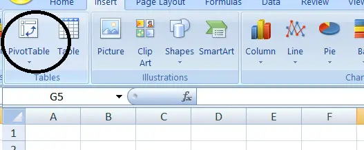
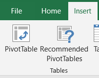
WHERE TO FIND THE PIVOT TABLE BUTTON LOCATION IN EXCEL?
We can find the option to insert PIVOT TABLES under the INSERT TAB under TABLES subsection.
BENEFITS OF USING PIVOT TABLES IN EXCEL
Let us discuss the benefits of using pivot tables and its uses in Excel.
Pivot tables are used when
- we need to analyze large data in a short notice.
- we need to total, summarize, category wise, sub category wise, perform different calculations like sum, average, or any custom calculation etc.
- A collapsible presentation, which we can twist and present in our own way within a few seconds.
- Play with rows and columns and create different reports.
- we need to filter, group, sort and conditionally format the data.
STEPS TO CREATE PIVOT TABLE IN EXCEL
Let us understand the steps to create pivot table using an example.
DATA SAMPLE:
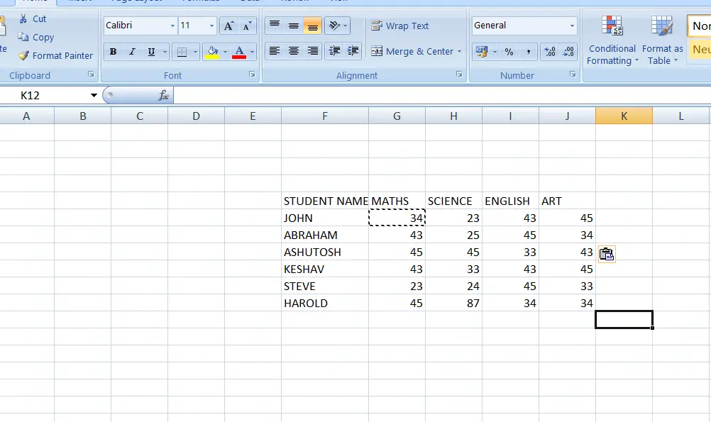
The pic below shows the sample data which we will be analyzing through PIVOT TABLES.
It shows a number of students with their marks in different subjects. Lets check what we can analyze through pivot.
The data in the table given can be copied by you to try on Excel.
| STUDENT NAME | MATHS | SCIENCE | ENGLISH | ART |
| JOHN | 34 | 23 | 43 | 45 |
| ABRAHAM | 43 | 25 | 45 | 34 |
| ASHUTOSH | 45 | 45 | 33 | 43 |
| KESHAV | 43 | 33 | 43 | 45 |
| STEVE | 23 | 24 | 45 | 33 |
| HAROLD | 45 | 87 | 34 | 34 |
STEPS TO CREATE A PIVOT TABLE:
- Select the data including headers ,go to insert tab and click PIVOT TABLE BUTTON.
STEPS TO CREATE A PIVOT TABLE:
- Click PIVOT TABLE BUTTON. A dialog box will open as shown in the following pic.
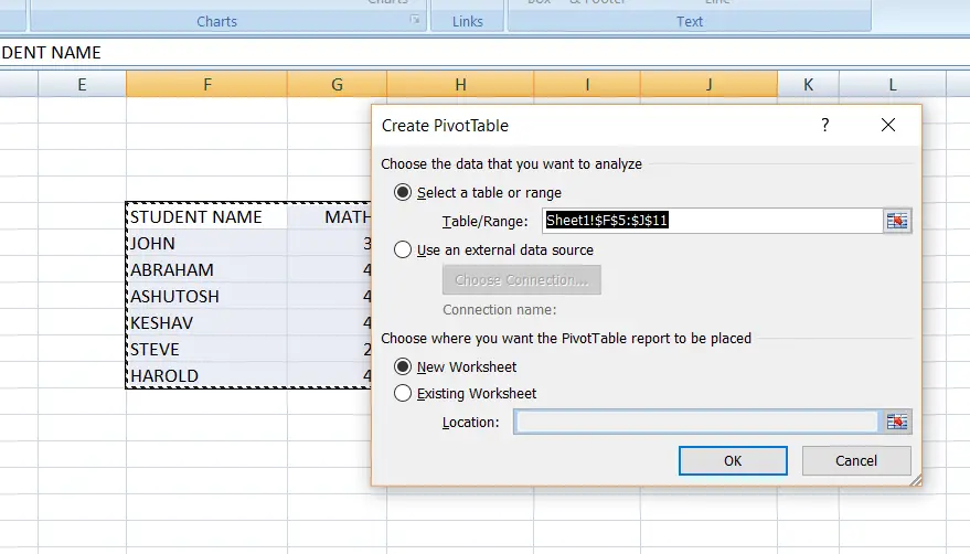
- As we have already selected the table, the range would show up automatically, otherwise we can put it manually or by selecting the table.
- Choose the location for the pivot tables. It can be on a NEW WORKSHEET or EXISTING WORKSHEET. If existing worksheet, we need to tell the starting cell location.
- CLICK OK.
- Our PIVOT TABLE is ready.
* We have discussed all the options in detail in the next portion of the article.
UNDERSTAND DIFFERENT OPTIONS AND SCREENS WHILE CREATING A PIVOT TABLE
Let us try to learn the different options available while creating the pivot tables.
CREATE PIVOT TABLE DIALOG BOX OPTIONS

Select a table or range: Enter the range manually or you can select it. We have already selected so a range will itself show in the box.
Use an external data source: Any external data source can also be used. It offers some online resources from various options. CLICK HERE TO KNOW MORE.
In the next options it asks whether you want the pivot table in a new worksheet or the existing one.

If you want in the existing one. Just give it the starting cell address and rest it’ll take care. Although it is always suggested to use the PIVOT TABLE in the new sheet so that it doesn’t mess up with our data.
After choosing the options, click OK.
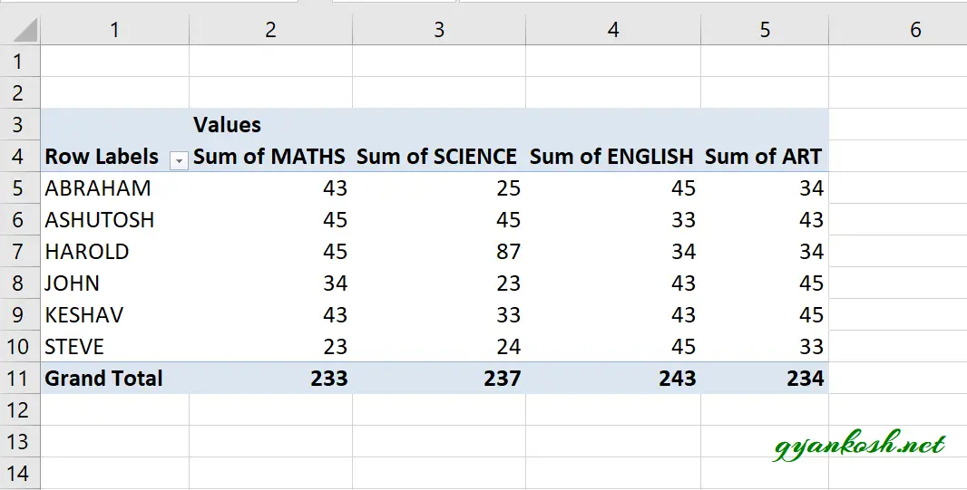
After clicking OK, it’ll create a pivot table, [Although not a table yet] , in a new sheet or the same sheet as per our preference. Below is the first screen of the pivot table containing sheet.
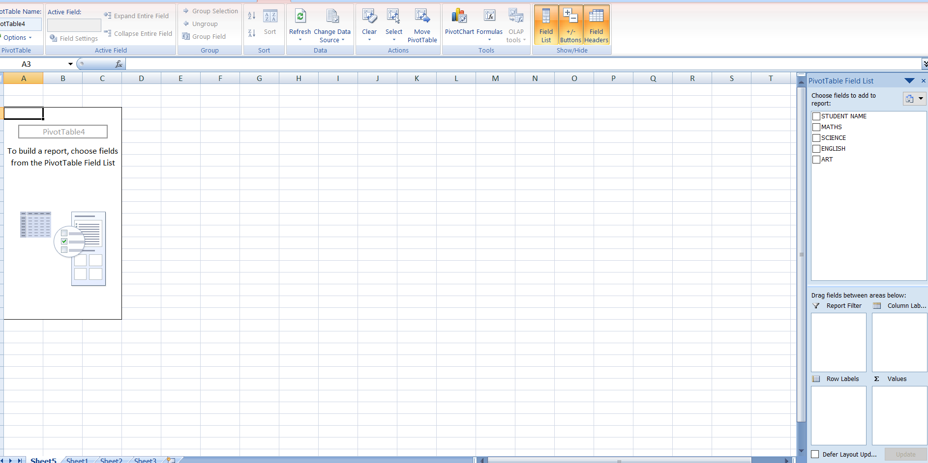
Click all the fields available on the right box named PIVOT TABLE FIELD LIST.Now let us understand the different areas of the PIVOT TABLE SHEET.
PIVOT TABLE SHEET DESCRIPTION IN EXCEL
DETAILS
Pivot table screen has the following area.
LOOK AT THE PICTURE BELOW FOR BETTER UNDERSTANDING.
Let us discuss all the areas one by one.
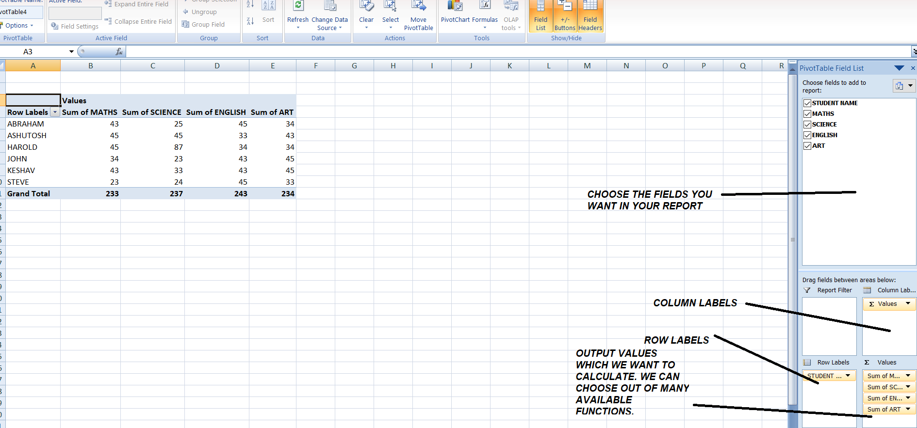
CHOOSE FIELDS TO ADD TO REPORT: This field consist of all the columns [fields] in the checkbox format.
Click the checkbox and that field will be used to create a table.
When we click it, Excel will automatically guess about its use and place it in any of the box. [Of course, we can change it as per requirement].
REPORT FILTER: It is an optional area. We can create filters there to keep the data we want. We can create a filter of any of the field and choose the data according to that.
COLUMN LABELS: This field will contain the columns of our pivot tables. For examples, if we need the values, we need to select values from the drop down list there.
ROW LABELS: The fields which we need as rows.
VALUES: The output values area. We need to specify the operation which must be put on our data so that we get the output.
We can select many operations in this field which we will see later in this article.
We put the fields in this area which we want to calculate.
CHANGE THE CALCULATION FORMULA IN PIVOT TABLE IN EXCEL
By default it started showing the total of all the values.
Lets explore the options present in the values (lower right) field.
Click the first one to choose the operation on the first column.
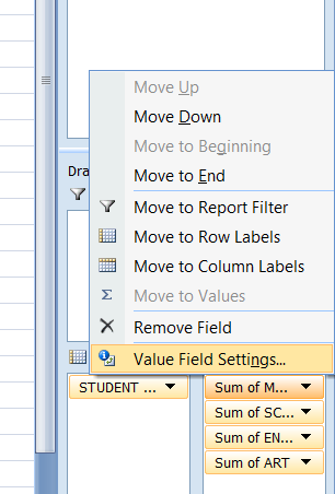
When clicked the option presents in VALUES the above shown box opens us. You can apply the options shows on the condition e.g. move to row labels or to column labels etc. or you can directly drag and drop also.
Lets go to VALUE FIELD SETTINGS.
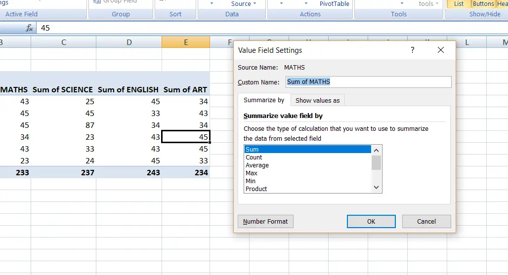
You can choose the NAME OF THE COLUMN and TYPE OF CALCULATION TO BE DONE.
Lets find out the average of the marks in first column.
Choose AVERAGE from the given list as shown in the picture above.
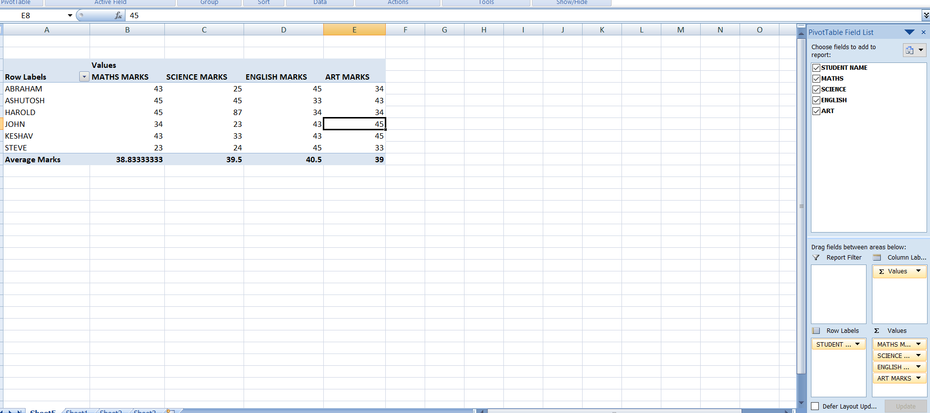
THE COLUMN AND ROW NAMES HAS BEEN CHANGED MANUALLY AS THE SYSTEM GIVES ITS OWN NAMES WHICH MAY NOT SUIT OUR REPORT.