Table of Contents
- INTRODUCTION
- WHERE IS FILTER DATA BUTTON IN EXCEL ?
- STEPS TO APPLY FILTER ON DATA IN EXCEL
- KEYBOARD SHORTCUT TO APPLY FILTER IN EXCEL
- WHEN TO USE FILTER ON DATA
- EXAMPLE TO APPLY A FILTER ON DATA
- FAQs
- HOW TO COPY FILTERED DATA IN EXCEL?
- CAN I APPLY TWO OR MORE SEPARATE FILTERS IN THE SAME SHEET?
- CAN I APPLY FILTER AND ADVANCED FILTER ON THE SAME SHEET AT THE SAME TIME?
- HOW TO FILTER DATA WITH A BUTTON?
- HOW TO COUNT THE FILTERED DATA IN EXCEL?
- OTHER WAYS TO FILTER THE DATA
INTRODUCTION
In practical applications, in maximum cases, we have a large data that can’t be managed by just having a look at the data and manually selecting it.
If we want to search for a particular data, we can do that by using control + F and then typing but it is again a cumbersome task to use it over and again and type the search word.
Or some other ways are to sort the data with respect to some column but in that case, too, we’ll need to eliminate the nonrequired data.
But after processing the concerned data this time, we again need to bring back the other data.
It is again not a very optimum way to manage the data.
So, for such situations, to analyze the data by just selecting a particular field and concentrating on concerning data only, we have got this option named FILTER.
Filtering the data is another one of the widely used options in EXCEL. It gives us the facility of instantly opting to see any particular class of data and seeing only what is needed.
WHERE IS FILTER DATA BUTTON IN EXCEL ?
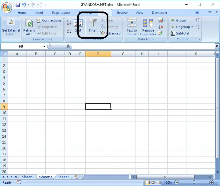
The button location for the FILTER OPTION is under the DATA TAB >SORT AND FILTER section.
The visual location is shown in the picture below.
STEPS TO APPLY FILTER ON DATA IN EXCEL
The following steps are used to apply a FILTER on any data.
STEPS:
- Go to DATA TAB>SORT AND FILTER section. The location is shown above in the picture.
- Select all the COLUMN HEADERS. The complete row can also be selected. It’ll apply filters only on the columns with data but if by chance there is some data in some unintended column, a filter will be given there also. So it is better to select the column headers only.
- Click FILTER BUTTON.
- The filter will be applied on the table.
- Take care that there is no gap between the headers and the data. The filter will be applied on all the contiguous ( Adjacent) data.
- The picture below shows the applied filter. The arrows appear in the lower right corner of the headers.
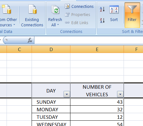
The above picture shows a FILTER APPLIED on the table. The arrows in the lower right corners show that the filter has been applied.
The data shows the number of vehicles sold on the days of a week.
KEYBOARD SHORTCUT TO APPLY FILTER IN EXCEL
There are countless keyboard shortcuts and we need not remember them all.
But even then if we are using any special operation quire a few times weekly, it is a good idea to start using the keyboard shortcuts.
It’s always faster than the mouse operation. So keyboard shortcut to apply a filter is
- Select the headers.
- Press ALT+A+T [Press ALT, A AND T SEQUENTIALLY. PRESS ALT, THEN A FIRST THEN T.]
.
WHEN TO USE FILTER ON DATA
Let us see in which conditions we should use filters on our data.
We can apply different types of operations on the filtered data such as sum, subtraction, etc. but the formulas should not be applied to the filtered data.
If formulas are applied, it takes into account all the rows hidden in between. But we can check the sum etc. or search for any specific information for the filtered data.
READ ME…
The filtering option just hides the rows which do not fulfill the conditions. So never apply any kind of operation. It’s just for analyzing the data.
EXAMPLE TO APPLY A FILTER ON DATA
LET’S UNDERSTAND THE DIFFERENT PROCEDURES OF FILTER USING A DATA SAMPLE.
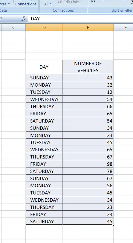
We have a number of vehicles delivered every day of the week for three weeks. Now let’s apply different filtering options to the data.
The given data is
| DAY | NUMBER OF VEHICLES |
| SUNDAY | 43 |
| MONDAY | 32 |
| TUESDAY | 12 |
| WEDNESDAY | 54 |
| THURSDAY | 66 |
| FRIDAY | 65 |
| SATURDAY | 54 |
| SUNDAY | 34 |
| MONDAY | 23 |
| TUESDAY | 45 |
| WEDNESDAY | 65 |
| THURSDAY | 67 |
| FRIDAY | 98 |
| SATURDAY | 78 |
| SUNDAY | 67 |
| MONDAY | 56 |
| TUESDAY | 45 |
| WEDNESDAY | 34 |
| THURSDAY | 23 |
| FRIDAY | 23 |
| SATURDAY | 45 |
STEPS TO APPLY FILTER
Here are the steps to apply filters to the given data.
- Select all the headers.
- Click FILTER button.
STEPS TO CHOOSE FROM AN APPLIED FILTER
Now, after the filter has been applied, let us see how to make the choices from the filters.
CLICK the arrow in the lower right corner of the filter header of the column, which you want to make the basis of filtering.
A list with the available options will open. Select the checkbox for the values you want to keep and uncheck the values you don’t want.
In the picture below, we are trying to look at the options available for the DAY COLUMN of the example.
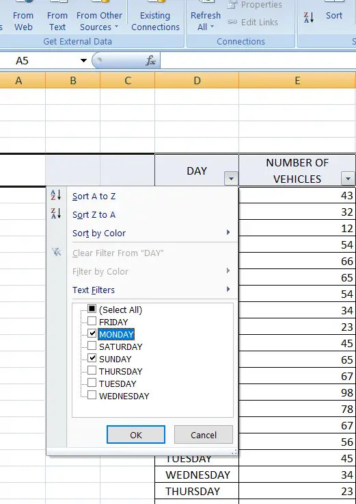
After clicking the drop-down of the filter, we can see that different options are there.
The options are the weekdays. We can choose any option from this list and only the chosen option and its counterparts in another column will remain.
The rest will be hidden.
If we want to check the vehicles on Monday and Sunday only, we uncheck the other days, as shown in the picture above and the result is shown in the next pic.
FAQs
HOW TO COPY FILTERED DATA IN EXCEL?
You can simply copy the data including the HEADINGS and paste it anywhere else.
The resulting data will be pasted only.
HOW TO FILTER DATA FOR CREATING CHARTS?
You can make use of the filters to create the dynamic charts which will produce the output as per the selected conditions.
FOLLOW THE STEPS TO CREATE THE DYNAMIC CHARTS USING FILTERS
- Apply the filter on the data table for the charts.
- Create the chart.
- The output of the chart will vary as per the filter condition applied.
CAN I APPLY TWO OR MORE SEPARATE FILTERS IN THE SAME SHEET?
No, as of now, it is not possible to apply more than one filter in a single sheet.
As soon as you apply the filter to some other data in the same sheet, it’ll remove the previous filter.
CAN I APPLY FILTER AND ADVANCED FILTER ON THE SAME SHEET AT THE SAME TIME?
No, you’ll be able to use only one FILTER or ADVANCED FILTER at the same time in one sheet. As soon as you apply the other option, the previous will be removed automatically.
HOW TO FILTER DATA WITH A BUTTON?
You won’t be able to create a proper macro with the help of FILTER OPTION but slicers are a better option to filter data with help of the ready-to-use buttons.
HOW TO COUNT THE FILTERED DATA IN EXCEL?
Yes, it is possible to count the filtered data in Excel. But, it won’t work with the FILTER UTILITY but FILTER FUNCTION.
After the output from the FILTER FUNCTION, apply the count formula on the result and it’ll provide you with the total count of the output.
LEARN COUNT FUNCTION HERE.
OTHER WAYS TO FILTER THE DATA
There are a few more options to get the same results. CLICK ANY OF THE OPTIONS.