Table of Contents
- INTRODUCTION
- What is the use of Xlookup function in Excel ?
- Prerequisites to learn Xlookup function in Excel
- What is syntax formula of Xlookup function in Excel?
- What are the benefits of using Xlookup function in Excel?
- EXAMPLE 1-How to use XLOOKUP function in Excel to extract a single value from data
- EXAMPLE 2-How to show custom error message using XLOOKUP function in Excel
- EXAMPLE 3-How to return multiple values using Xlookup function in Excel
- EXAMPLE 4- How to search a value nearest to the other value using Xlookup in Excel
- EXAMPLE 5-How to use Nested Xlookup in Excel
INTRODUCTION
XLOOKUP FUNCTION is a new function introduced in some of the EXCEL OPTIONS, such as EXCEL 365, EXCEL FOR ANDROID ETC.
We make and manage large report in Excel. Many times we need to join two or more reports into a final single report but would that be possible if there are hundreds of lines in all the three reports.
The Answer is NO!!!
But thanks to excel, which has given us many ways to help joining of such reports. Two of these options are HLOOKUP AND VLOOKUP. And one more very powerful option, which is similar to VLOOKUP but have many additional functions is XLOOKUP. (But available in few MICROSOFT OPTIONS only)
THIS ARTICLE DEALS WITH XLOOKUP.
What is the use of Xlookup function in Excel ?
XLOOKUP helps to retrieve an array of values from a table. It is a way in Excel to find out and extract a set of values by matching any value of the table.
XLOOKUP IS AN OFFICE 365 FUNCTION WHICH HELPS US TO LOOK UP FOR A VALUE AND RETRIEVE ANY OTHER VALUE OR A COMPLETE ARRAY OF VALUES AGAINST THE LOOKED UP VALUE.
Prerequisites to learn Xlookup function in Excel
THERE ARE A FEW PREREQUISITES WHICH WILL ENABLE YOU TO UNDERSTAND THIS FUNCTION IN A BETTER WAY.
- Basic understanding of how to use a formula or function.
- Easier to understand if user already knows how to use HLOOKUP OR VLOOKUP.
- Basic understanding of rows and columns in Excel.
- Of course, Excel software.
Helpful links for the prerequisites mentioned above
What Excel does? How to use formula in Excel?
What is syntax formula of Xlookup function in Excel?
The syntax ( the way how formula is phrased for excel) of XLOOKUP is
=XLOOKUP (VALUE TO BE FOUND , LOOKUP TABLE , RETURN ARRAY , ERROR MESSAGE , MATCH MODE , SEARCH MODE )
VALUE TO BE FOUND The value to be found and matched
LOOKUP TABLE The range of cells, where we will try to find the match
RETURN ARRAY The returning array or a set of values to be returned after the match has been made
ERROR MESSAGE If value is not found, this message will be displayed. Its kind of error handling.
MATCH MODE
0 – Exact match. If none found, return #N/A. This is the default.
-1 – Exact match. If none found, return the next smaller item.
1 – Exact match. If none found, return the next larger item.
2 – A wildcard match where *, ?, and ~ have special meaning.
SEARCH MODE
1 – Perform a search starting at the first item. This is the default.
-1 – Perform a reverse search starting at the last item.
2 – Perform a binary search that relies on LOOKUP VALUE being sorted in ascending order. If not sorted, invalid results will be returned.
-2 – Perform a binary search that relies on LOOKUP VALUE being sorted in descending order. If not sorted, invalid results will be returned.
What are the benefits of using Xlookup function in Excel?
No need to specify column index: Unlike VLOOKUP, XLOOKUP doesn’t require you to define the column number from which to return a value.
Search in any direction: XLOOKUP can look both left-to-right and right-to-left, unlike VLOOKUP which can only search left-to-right.
Wildcard and exact match: You can use wildcards, exact matches, and other types of matching more flexibly.
Error handling: With the [if_not_found] argument, you can control what happens if a match isn’t found.
EXAMPLE 1-How to use XLOOKUP function in Excel to extract a single value from data
OBJECTIVE
The data sample contains a table with the different details of the employees such as email id, date of birth(DOB), salary and experience.The first example shows the simple lookup from the table and returning the value as we use to do in the VLOOKUP.Here is the given table.*The table which can be copied directly to the sheet is available when you see the page in desktop or tablet.
| GYANKOSH.NET | ||||
| NAME | EMAIL ID | DOB | SALARY | EXPERIENCE |
| MICHAEL | michael@abc.com | 12.02.1990 | 12000 | 10 |
| RAVI | ravi@abc.com | 15.03.1991 | 10000 | 1 |
| DANIEL | daniel@abc.com | 14.05.2013 | 30000 | 2 |
| FLORENCE | florence@abc.com | 18.06.2000 | 45000 | 5 |
| TOM | tom@abc.com | 25.07.2001 | 98000 | 4 |
| HARRY | harry@abc.com | 31.7.1993 | 65000 | 6 |
The details can be seen . For the example, the table taken is small so that we can verify the working of the formula too. In practical reports table goes upto hundreds of thousands of rows. The efficacy of the formula will still be same.Check out the animation below which shows the use of xlookup to find out the salary of the employee named DANIEL.
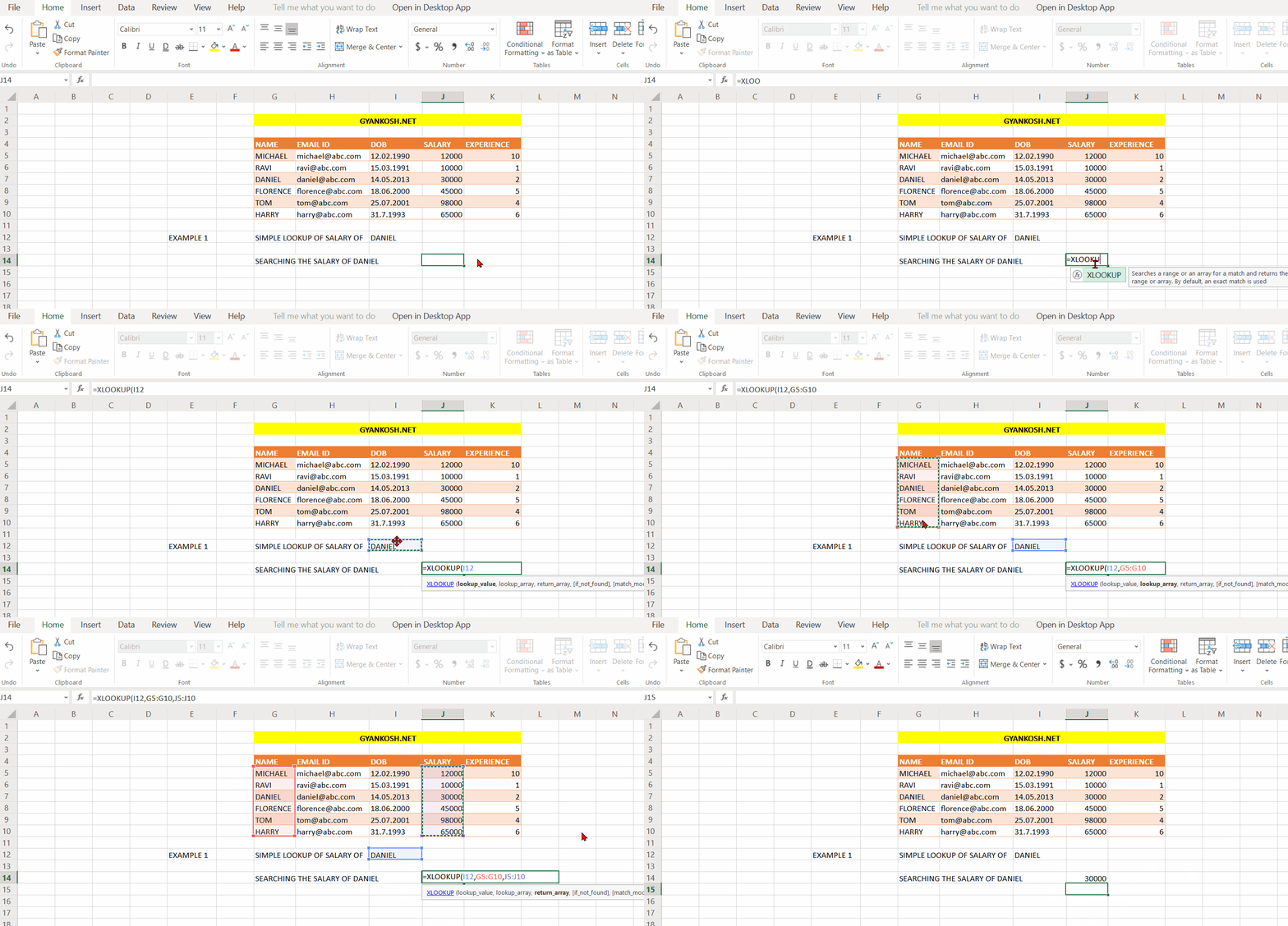
STEPS TO USE XLOOKUP – EXAMPLE 1
1. Place the cursor in the cell where we want to get the result. For the example, place the cursor in J14.
2. Type the formula
=XLOOKUP(I12,G5:G10,J5:J10)
3. Click ENTER and the result will appear as 30000 , WHICH IS THE SALARY OF DANIEL.
EXPLANATION OF STEPS- EXAMPLE 1
The formula used is
=XLOOKUP(I12,G5:G10,J5:J10)I12, first argument, contains the value to be found which is DANIEL in this case.Second argument G5:G10 contains the array from which the value DANIEL is to be found.tHIRD ARGUMENT, J5:J10, contains the values which needs to be returned or which we need.REST OF THE ARGUMENTS ARE OPTIONAL AND NOT USED IN THIS EXAMPLE.
DO YOU KNOW
XLOOKUP IS JUST LIKE VLOOKUP BUT MORE POWERFUL. IT CAN RETURN A COMPLETE ARRAY OF RESULTS IN ONE GO.
EXAMPLE 2-How to show custom error message using XLOOKUP function in Excel
OBJECTIVE
The data sample contains a table with the different details of the employees such as email id, date of birth(DOB), salary and experience.The first example shows the simple lookup from the table and returning the value as we use to do in the VLOOKUP.
In this example
WE’LL MAKE USE OF THE PARTICULAR INPUT AVAILABLE IN XLOOKUP FOR CUSTOM ERROR MESSAGE. THE MESSAGE DISPLAYED IN CASE THE VALUE IS NOT FOUND.
Here is the given table.
*The table which can be copied directly to the sheet is available when you see the page in desktop or tablet.
| GYANKOSH.NET | ||||
| NAME | EMAIL ID | DOB | SALARY | EXPERIENCE |
| MICHAEL | michael@abc.com | 12.02.1990 | 12000 | 10 |
| RAVI | ravi@abc.com | 15.03.1991 | 10000 | 1 |
| DANIEL | daniel@abc.com | 14.05.2013 | 30000 | 2 |
| FLORENCE | florence@abc.com | 18.06.2000 | 45000 | 5 |
| TOM | tom@abc.com | 25.07.2001 | 98000 | 4 |
| HARRY | harry@abc.com | 31.7.1993 | 65000 | 6 |
The details can be seen . For the example, the table taken is small so that we can verify the working of the formula too. In practical reports table goes upto hundreds of thousands of rows. The efficacy of the formula will still be same.Check out the animation below which shows
that we are trying to find out the salary of an employee named MADRI.
As we know that no such employee exist, the formula returns the custom error, “EMPLOYEE NOT FOUND”.
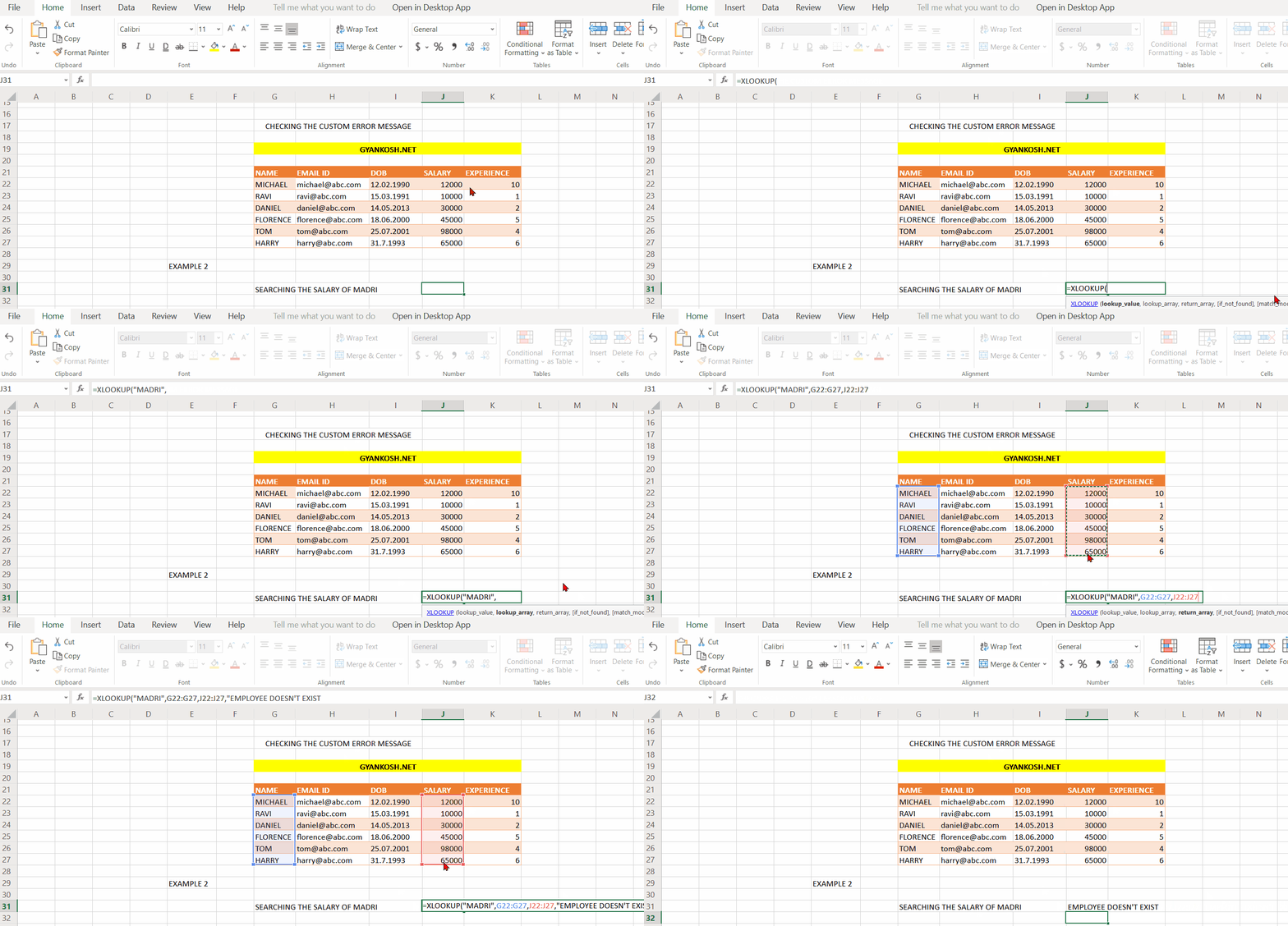
STEPS TO USE XLOOKUP – EXAMPLE 2
1. Place the cursor in the cell where we want to get the result. For the example, place the cursor in J14.
2. Type the formula
=XLOOKUP(I12,G5:G10,J5:J10)
3. Click ENTER and the result will appear as 30000 , WHICH IS THE SALARY OF DANIEL.
EXPLANATION OF STEPS- EXAMPLE 2
The formula used is
=XLOOKUP (“MADRI”, G28:G33 , J28:J33 , “EMPLOYEE DOESN’T EXIST” )
“MADRI”, first argument, contains the value to be found. MADRI is the name of the employee whose details we want to get.
Second argument G28:G33 contains the array from which the value MADRI is to be found.
THIRD ARGUMENT, J28:J33, contains the values which needs to be returned or which we need.
REST OF THE ARGUMENTS ARE OPTIONAL AND NOT USED IN THIS EXAMPLE.
FOURTH ARGUMENT GOES AS THE “ERROR MESSAGE”.
The message which we want to be displayed if a value is not found. In this case it is “EMPLOYEE NOT FOUND” which is displayed as the result.
EXAMPLE 3-How to return multiple values using Xlookup function in Excel
OBJECTIVE
The data sample contains a table with the different details of the employees such as email id, date of birth(DOB), salary and experience.THIS FUNCTION DIFFERS MAINLY FROM VLOOKUP AS IT CAN RETURN A COMPLETE ARRAY IN THE SINGLE GO. Here is the given table.
*The table which can be copied directly to the sheet is available when you see the page in desktop or tablet.
| GYANKOSH.NET | ||||
| NAME | EMAIL ID | DOB | SALARY | EXPERIENCE |
| MICHAEL | michael@abc.com | 12.02.1990 | 12000 | 10 |
| RAVI | ravi@abc.com | 15.03.1991 | 10000 | 1 |
| DANIEL | daniel@abc.com | 14.05.2013 | 30000 | 2 |
| FLORENCE | florence@abc.com | 18.06.2000 | 45000 | 5 |
| TOM | tom@abc.com | 25.07.2001 | 98000 | 4 |
| HARRY | harry@abc.com | 31.7.1993 | 65000 | 6 |
The details can be seen .
For the example, the table taken is small so that we can verify the working of the formula too.
In practical reports table goes upto hundreds of thousands of rows. The efficacy of the formula will still be same.
Check out the animation below which shows the
use of xlookup to LOOKUP FOR A VALUE AND RETURN AN ARRAY OF MORE THAN ONE INFORMATION IN A SINGLE FORMULA.
We will try to get the salary and experience of the employee named RAVI.
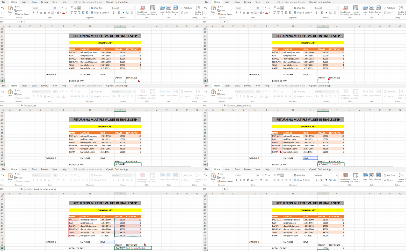
STEPS TO USE XLOOKUP – EXAMPLE 3
1. Place the cursor in the cell where we want to get the result. For the example, place the cursor in J54.
2. Type the formula
=XLOOKUP(I58,G51:G56,J51:K56)
3. Click ENTER and the result will appear as 10000 and 1 , WHICH ARE THE SALARY AND EXPERIENCE OF RAVI.
EXPLANATION OF STEPS- EXAMPLE 3
The formula used is
=XLOOKUP(I58,G51:G56,J51:K56)I58,which have
RAVI value, first argument, contains the value to be found. RAVI is the name of the employee whose details we want to get.
Second argument G51:G56 contains the array from which the value RAVI is to be found.
THIRD ARGUMENT, J51:K56, contains the values which needs to be returned or which we need. Here we can see that the third argument contains two columns. The values from these two columns will be returned. Similarly we can take any number of columns to be returned.
REST OF THE ARGUMENTS ARE OPTIONAL AND NOT USED IN THIS EXAMPLE.
EXAMPLE 4- How to search a value nearest to the other value using Xlookup in Excel
OBJECTIVE
The data sample contains a table with the different details of the employees such as email id, date of birth(DOB), salary and experience.VLOOKUP doesn’t give us the option of specifying the matching mode, where we can match the value, or we can go to next higher or lower value as per the requirement but here we do have such liberty. In this example we will try MATCHING MODE , the fifth argument.Here is the given table.*The table which can be copied directly to the sheet is available when you see the page in desktop or tablet.
| GYANKOSH.NET | ||||
| NAME | EMAIL ID | DOB | SALARY | EXPERIENCE |
| MICHAEL | michael@abc.com | 12.02.1990 | 12000 | 10 |
| RAVI | ravi@abc.com | 15.03.1991 | 10000 | 1 |
| DANIEL | daniel@abc.com | 14.05.2013 | 30000 | 2 |
| FLORENCE | florence@abc.com | 18.06.2000 | 45000 | 5 |
| TOM | tom@abc.com | 25.07.2001 | 98000 | 4 |
| HARRY | harry@abc.com | 31.7.1993 | 65000 | 6 |
The details can be seen . For the example, the table taken is small so that we can verify the working of the formula too. In practical reports table goes up to hundreds of thousands of rows. The efficacy of the formula will still be same.Check out the animation below which shows the use of xlookup to find out a value nearest to the next higher or next lower value.
IN THIS EXAMPLE WE’LL FIND OUT THAT WHICH EMPLOYEE HAS THE SALARY NEAR TO 40000 IN BOTH DIRECTIONS .
UPPER AND LOWER.
LET US CHECK HOW TO USE XLOOKUP FOR THAT.
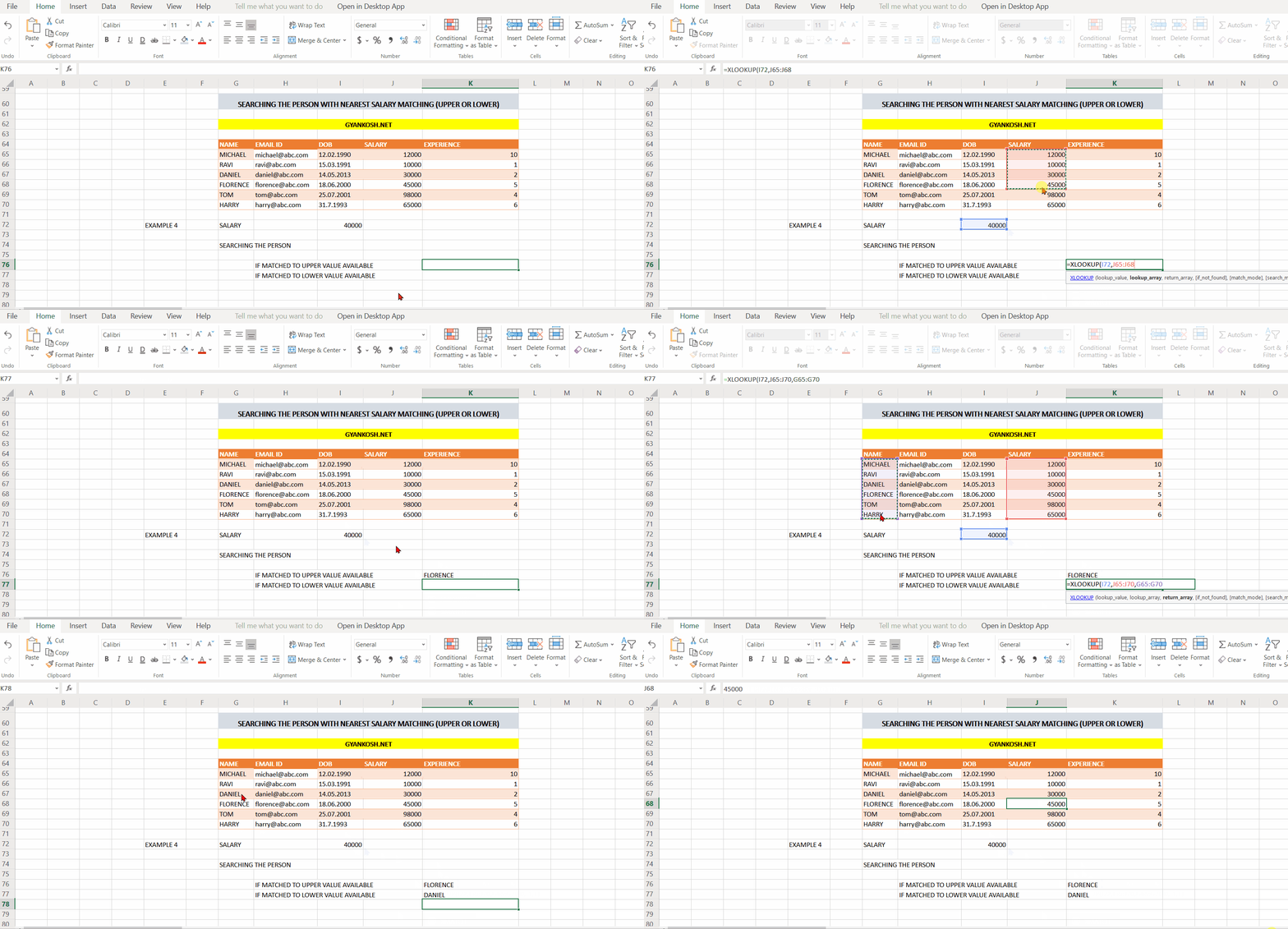
STEPS TO USE XLOOKUP – EXAMPLE 4
1. Place the cursor in the cell where we want to get the result. For the example, place the cursor in J14.
FOR UPPER VALUE AVAILABLE
2. Type the formula
=XLOOKUP(I72,J65:J70,G65:G70,0,1,1)
3. Click ENTER and the result will appear as FLORENCE, which is obvious as the MATCHING MODE is 1, which means that it’ll find out the next higher value if matching value is not found. so salary of florence is 45000 and the answer is correct.
FOR LOWER VALUE AVAILABLE
Type the formula
=XLOOKUP(I72,J65:J70,G65:G70,0,-1,1)
4.Click ENTER and the result will appear as DANIEL, which is obvious as the MATCHING MODE is -1, which means that it’ll find out the next higher value if matching value is not found. so salary of DANIEL is 30000 and
the answer is correct.
EXPLANATION OF STEPS- EXAMPLE 4
The two function used for the UPPER VALUE ADAPTION and LOWER VALUE ADAPTION are as follows
FOR UPPER VALUE
=XLOOKUP(I72,J65:J70,G65:G70,0,-1,1)
FOR LOWER VALUE
=XLOOKUP(I72,J65:J70,G65:G70,0,-1,1)
As we can see that there is just one difference between the two functions used is the ARGUMENT NO. 5 i.e. matching mode. we’ll discuss it later in the same para.
I72 contains the value 40000, which we need to match with the salaries of employees. We’ll do it in two ways when we’ll match the salary to the next higher and to the next lower salaries available.
Second argument J65:J70 is the range of the salaries of employees from where it’ll fix the answer row.
Third argument is G65:G70, which will be returned as result after doing the match.
FOURTH ARGUMENT is given as 0, which is the customized error message and will return a 0 if it doesn’t find the required value.
FIFTH ARGUMENT is 1 and -1 which completely changes our results.As 1 matching mode, it’ll return the exact match or next higher value which is 45000 and FLORENCE has that salary so the answer is FLORENCE.Similarly when MATCHING MODE is -1, it’ll return the exact match or next lower which is 30000 and it is the salary of DANIEL, which is shown as ANSWER.
EXAMPLE 5-How to use Nested Xlookup in Excel
OBJECTIVE
The data sample contains a table with the different details of the employees such as email id, date of birth(DOB), salary and experience.
This example shows the nested usage of XLOOKUP along with SUM AND LARGE FUNCTIONS.
*The table which can be copied directly to the sheet is available when you see the page in desktop or tablet.
| GYANKOSH.NET | ||||
| NAME | EMAIL ID | DOB | SALARY | EXPERIENCE |
| MICHAEL | michael@abc.com | 12.02.1990 | 12000 | 10 |
| RAVI | ravi@abc.com | 15.03.1991 | 10000 | 1 |
| DANIEL | daniel@abc.com | 14.05.2013 | 30000 | 2 |
| FLORENCE | florence@abc.com | 18.06.2000 | 45000 | 5 |
| TOM | tom@abc.com | 25.07.2001 | 98000 | 4 |
| HARRY | harry@abc.com | 31.7.1993 | 65000 | 6 |
The details can be seen . For the example, the table taken is small so that we can verify the working of the formula too. In practical reports table goes upto hundreds of thousands of rows. The efficacy of the formula will still be same.Check out the animation below which shows the use of xlookup to find out the sum of experience of two highest paid employees. Here, as the table is small, we can see that highest paid employees are TOM and HARRY and the sum of their experience is 10 years. Let us try to get that with the help of XLOOKUP.
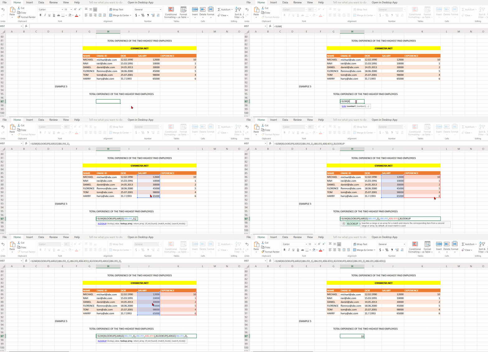
STEPS TO USE XLOOKUP – EXAMPLE 5
This objective can be achieved with the following steps.
First of all, we need to find out the highest paid employees for which we will use the LARGE FUNCTION.
Second step is to find out the EXPERIENCE of the two found employees.
Finally the sum of both.So here are the steps.
1. Place the cursor in the cell where we want to get the result. For the example, place the cursor in J97.
2. Type the formula
=XLOOKUP(I12,G5:G10,J5:J10)
3. Click ENTER and the result will appear as 30000 , WHICH IS THE SALARY OF DANIEL.
EXPLANATION OF STEPS- EXAMPLE 5
The formula used is
=SUM(XLOOKUP (LARGE (J86:J91,1) , J86:J91 , K86:K91 ) , XLOOKUP (LARGE(J86:J91,2) , J86:J91 , K86:K91))
The outermost function used is SUM. inside that we start with the XLOOKUP where we will be getting the experience of two highest paid persons.
In the xlookup, the lookup value is taken through the LARGE FUNCTION which goes as LARGE(J86:J91,1) which means that we have to find the highest salary from the column of salaries.
Similarly in the second XLOOKUP, we’ll find the second highest salary by using LARGE(J86:J91,2).
These two salaries will go for the look up value in the Second argument of XLOOKUP which is the salary array as J86:J91.
After pinpointing these salaries, the value returning array is the experience column which is K86:K91.
The returning value of both XLOOKUPS comes out to be 4 and 6.
These values work as the argument for the outermost SUM FUNCTION and total comes out to be 10 as the answer. We achieved the goal.
Similarly we can use many functions together to perform complex functions.