HLOOKUP is as advanced level function. But advanced doesn’t mean tough. In this article we’ll try to find out what we can do with this function and how to use it.
We make and manage large report in Excel. Many times we need to search for a value from a big report or join two or more reports into a final single report but would that be possible if there are hundreds of lines in all the three reports.
The Answer is NO!!!
But thanks to excel, which has given us many ways to help joining of such reports. Two of these options are HLOOKUP AND VLOOKUP.
THIS ARTICLE DEALS WITH HLOOKUP, which is used a bit less than VLOOKUP.
PURPOSE OF HLOOKUP IN EXCEL
HLOOKUP provides us a way to retrieve a value present in the same column of the value to be found ,from a selected table, by matching the “Value to be found” in the first row of the selected table.
Kindly read the statement twice as may seem to be confusing at first.
Suppose we have a horizontal table in which the headings are in the first row and details are in vertical columns. Now if we need to extract any data, we’ll search for the first row of the selected table and after matching the column heading, we can retrieve any value against that particular column. It’ll become very clear after we discuss the example.
PREREQUISITES TO LEARN HLOOKUP
THERE ARE A FEW PREREQUISITES WHICH WILL ENABLE YOU TO UNDERSTAND THIS FUNCTION IN A BETTER WAY.
- Basic understanding of how to use a formula or function.
- Basic understanding of rows and columns in Excel.
- Of course, Excel software.
Helpful links for the prerequisites mentioned aboveWhat Excel does? How to use formula in Excel?
SYNTAX: HLOOKUP FUNCTION
The syntax ( the way how formula is phrased for excel) of HLOOKUP is
=HLOOKUP(cell address of value to be matched , range of cells to search , row number to return the value, match should be approximate or exact)
So, a sample format is here. Suppose the value to be found is in cell H13 and the table from which the value is to be extracted has the range I12:K25 (14 rows) and the match is to be exact.The format in the output cell will be
=hlookup(H13,I12:K25,6,false)
This will find out the value of H13 in the table I12:K25 and return the value of sixth row i.e. I17 if it could find H13 in the table’s first row.
EXAMPLE : HLOOKUP IN EXCEL (EXTRACTING A SINGLE VALUE FROM DATA)
DATA SAMPLE
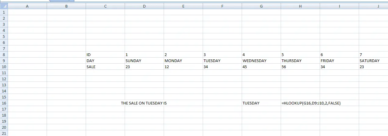
The sample data shows sales number for a week. Data is arranged horizontally and the objective is to find the sales on Tuesday.
Apply the formula of HLOOKUP on the cell H16.
Type in H16
=HLOOKUP(G16,D9:J10,2,FALSE) as mentioned in the picture.

STEPS TO USE HLOOKUP
- We will make use of HLOOKUP as our data is in landscape format.
- As per the syntax,
- =HLOOKUP(cell address of value to be matched, range of cells to search, row number to return the value, match should be approximate or exact )
- PUT in cell H16 , the following formula “=hlookup( (G16,D9:J10,2,FALSE) ” (“” shouldn’t be written in the formula bar”)
- Press ENTER.
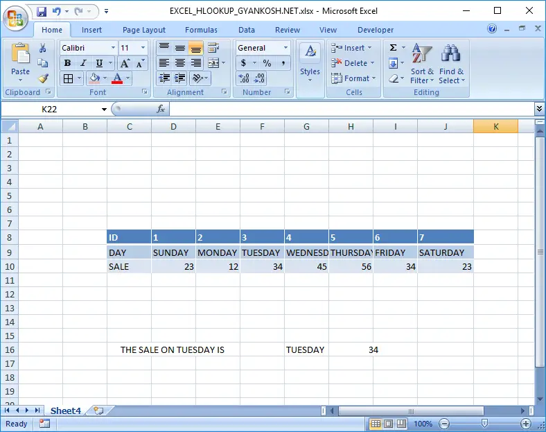
- “34” will appear in the cell, as expected.
- The output screen is shown.

STEP WISE STEP EXPLANATION
LET US UNDERSTAND HOW THE FORMULA WAS INTERPRETED BY THE EXCEL.
=hlookup( (G16,D9:J10,2,FALSE)
WORDWISE BREAKUP OF FORMULA
| EXPLANATION OF THE FORMULA USED | |
|---|---|
| = | EVERY FORMULA STARTS WITH AN “=” |
| HLOOKUP | FUNCTION NAME |
| G16 | The value to be found. In this case, DAY is a unique value which we will be using. With the help of this UNIQUE VALUE we’ll help Excel to search out our desired value and return it to us. |
| D9:J10 | Range in which excel will find G16 value. The range is the top left cell upto the bottom right cell of the table. |
| FALSE | Exact Match. True is used for Approximate Match |
CONFUSION CLARIFICATIONS
ROW INDEX NUMBER (INPUT NO. 3 IN HLOOKUP FORMULA)
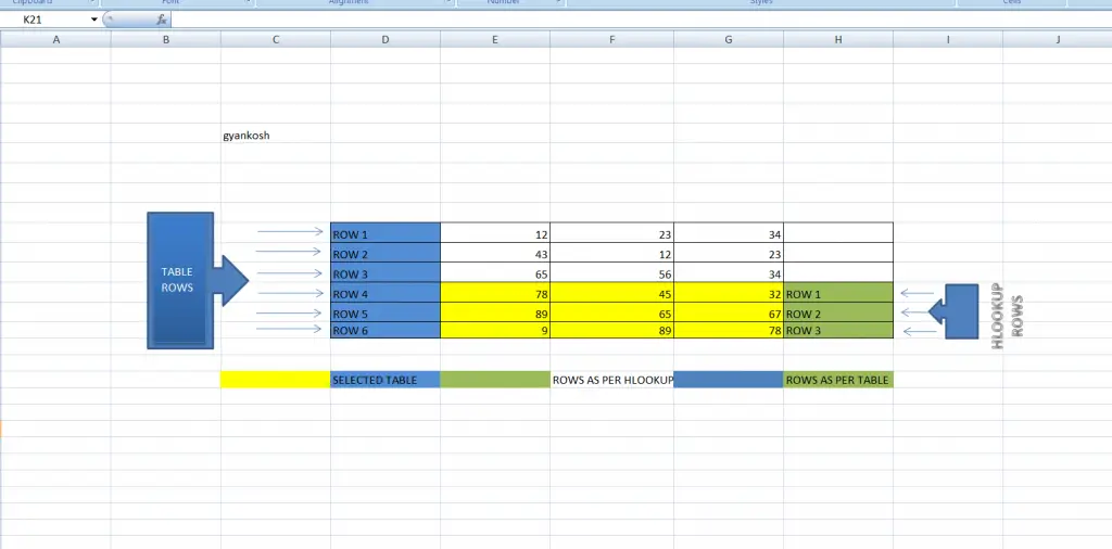
Its very easy to understand. The Range, which has been selected by us to find our desired value from, is considered a table by the excel and its ROW NUMBERS will be counted from top to bottom irrespective of the original table.
EXAMPLE:
Checkout the illustration given in the picture.
The Range selection area is colored in YELLOW.
The table has six rows but for HLOOKUP, the rows will be counted from the first row at the top of selected range as shown by GREEN arrows.
