Table of Contents
- INTRODUCTION
- PURPOSE OF VLOOKUP IN GOOGLE SHEETS
- PREREQUISITES TO LEARN VLOOKUP
- SYNTAX: VLOOKUP FUNCTION IN GOOGLE SHEETS
- EXAMPLE 1:VLOOKUP IN GOOGLE SHEETS (EXTRACTING A SINGLE VALUE FROM DATA)
- EXAMPLE 2: HOW TO LOOKUP AND RETRIEVE MULTIPLE DATA USING VLOOKUP IN GOOGLE SHEETS
- CONFUSION CLARIFICATIONS
INTRODUCTION
Welcome to the step by step guide to VLOOKUP in GOOGLE SHEETS. The article covers the introduction , basics of Vlookup as well as all the different usages of vlookup using the examples.
VLOOKUP is one of the most useful functions of GOOGLE SHEETS and is treated as an advanced level function. But advanced doesn’t mean tough. In this article we’ll try to find out what we can do with this function and how to use it. It’ll be a step wise step introduction to the Vlookup.
We prepare and manage large reports in SPREADSHEET SOFTWARES. Many times we need to join or consolidate two or more reports into a final single report but would that be possible if there are hundreds of lines in all the reports to be joined.
The Answer is NO!!!
But thanks to lookup and retrieving functions like VLOOKUP, which has given us many ways to help joining of such reports.
The article will start with the purpose of VLOOKUP, after which examples using different options will be taken.
PURPOSE OF VLOOKUP IN GOOGLE SHEETS
“VLOOKUP enables us to LOOKUP for a particular value or text from another TABLE and return ANY value from the cells of the same row of that looked up value. “
EXAMPLE: Kindly read it for the concept building if you are a first time user.
We have a list of ROLL NUMBER of the students in a class with their names.
There is another table with ROLL NUMBERS and the complete details of the students such as NAME, ADDRESS, STANDARD etc.
Now if we want to find out any details of the students such as ADDRESS. We’ll do that by using VLOOKUP.
VLOOKUP needs a unique identifying field i.e. some value/text which is present in both the places, the looker and the table from where the item will be looked up.
Here ROLL NO. is that identifier.
After looking up the ROLL NO. we can retrieve any value present against that ROLL NO. in that table such as NAME, ADDRESS , STANDARD etc.
This is the use of VLOOKUP.
PREREQUISITES TO LEARN VLOOKUP
THERE ARE A FEW PREREQUISITES WHICH WILL ENABLE YOU TO UNDERSTAND THIS FUNCTION IN A BETTER WAY.
- Basic understanding of how to use a formula or function.
- Basic understanding of rows and columns in GOOGLE SHEETS.
- Of course, access to GOOGLE SHEETS.
SYNTAX: VLOOKUP FUNCTION IN GOOGLE SHEETS
The syntax ( the way how formula is phrased for google sheets) of VLOOKUP is
=VLOOKUP(cell address of value to be matched, range of cells to search, column number to return the value, If the data is sorted or not which corresponds to approximate match or exact match)
So, a sample format is here. Suppose the value to be found is in cell H13 and the table from which the value is to be extracted has the range I12:K25 (3 columns) and the match is to be exact.The format in the output cell will be
=vlookup(H13,I12:K25,3,false)
This will find out the value of H13 in the table I12:K25 and return the value of third column i.e. K if it could find H13 in the table’s first column.
If you didn’t understand this, don’t worry, we’ll solve a few examples for better understanding.
EXAMPLE 1:VLOOKUP IN GOOGLE SHEETS (EXTRACTING A SINGLE VALUE FROM DATA)
DATA SAMPLE
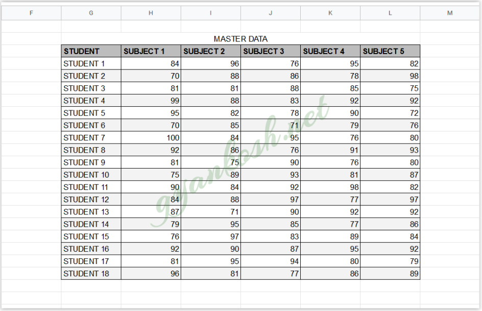
We have a master data of a class of few students containing their marks in the different subjects.
Let us try to find out the MARKS OF STUDENT 10 IN THE SUBJECT 3.
This is the demonstration of the simple lookup using the VLOOKUP FUNCTION.
Following picture shows the available master data.
OBJECTIVE
TO FIND OUT THE MARKS SECURED BY STUDENT 10 IN SUBJECT 3 USING THE VLOOKUP FUNCTION
STEPS TO APPLY VLOOKUP
- As per the syntax, the VLOOKUP function has the following syntax
- =VLOOKUP(cell address of value to be matched, range of cells to search, column number to return the value, match should be approximate or exact
- PUT in cell D7 , the following formula =VLOOKUP(“STUDENT 10”,G6:L23,4,FALSE) .(FOR REFERRING THE CELLS OF THE TABLES, USE THE NEXT PICTURE WHICH SHOWS THE CELL NUMBERS.)
- Press ENTER. “93” will appear in the cell, as expected. [ The answer is correct which can be manually checked ].
- The output screen is shown.
*The step wise step explanation follows after the picture.
STEP WISE STEP EXPLANATION
LET US UNDERSTAND HOW THE FORMULA WAS INTERPRETED BY THE GOOGLE SHEETS.
==VLOOKUP(“STUDENT 10”,G6:L23,4,FALSE)
WORDWISE BREAKUP OF FORMULA
| EXPLANATION OF THE FORMULA USED | |
|---|---|
| = | EVERY FORMULA STARTS WITH AN “=” |
| VLOOKUP | FUNCTION NAME |
| “STUDENT 10” | The value to be found. In this case, ROLL NO. is a unique value which is present in both the tables. With the help of this UNIQUE VALUE we’ll help GOOGLE SHEETS to search out our desired value and return it to us. |
| G6:L23 | Range in which GOOGLE SHEETS will find J21 value. The range is the top left cell upto the bottom right cell of the table. |
| FALSE | EXACT MATCH. False is used for exact match or when the data is not sorted. |
The result comes out to be 93.
EXAMPLE 2: HOW TO LOOKUP AND RETRIEVE MULTIPLE DATA USING VLOOKUP IN GOOGLE SHEETS
LOOKING AND RETRIEVING VALUES FROM A LONG LIST
Let us extend our example 1 to a more practical scenario and learn the way to sort the problem easily.
The following picture shows the same table [ Trimmed a bit at the bottom ].
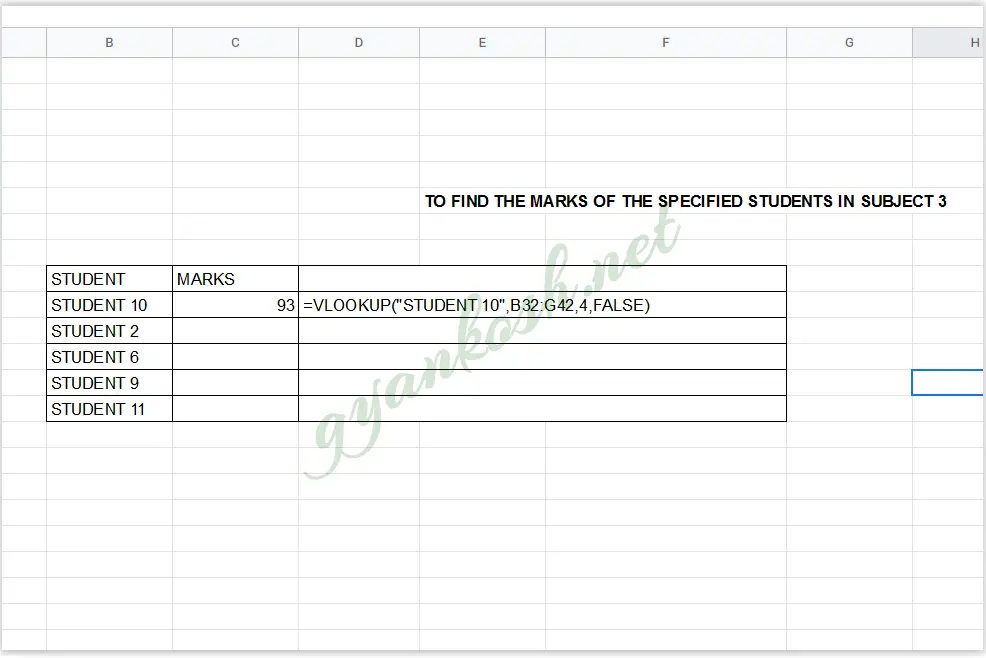
Now, instead of a single student we have a random list of students and we need to find the marks of these students from the master table
SOLUTION
Have a look at the table given above.
WE WANT TO LOOK UP THE MARKS OF ALL THE GIVEN STUDENTS
We have already looked up the marks of STUDENT 3.
Let us just drag down the same formula and check if it works for us or not.
After dragging down the formula, the table becomes like this.
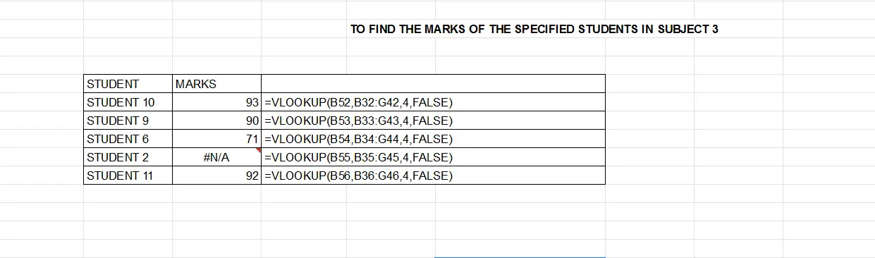
In the table above, when we dragged down the formula, We got a N/A error against the STUDENT 2 which is not desired.
The reason for this error is the way Google Sheets behavior when we drag any formula.
When we drag the formula, the reference addresses are changed to keep them relatively intact but it creates the problem in the lookup cases as the TABLE TO BE LOOKED UP values will change too which will make few of the vales showing N/A [ VALUE NOT AVAILABLE ] error.
After dragging down the formula, the table becomes like this.
TO TACKLE SUCH CASE, WHEN WE NEED TO DRAG A VLOOKUP FORMULA
THROUGH A BIG NUMBER OF ROWS, WE NEED TO FIX THE CELL RANGE [ LOOKUP RANGE ]
AS WHEN WE DRAG, THE CELL RANGE ALSO STARTS CHANGING RELATIVELY.
DO YOU KNOW
GOOGLE SHEETS FORMULAS WORKS RELATIVELY. IF WE DRAG ANY FORMULA, IT’LL CHANGE THE CELL ADDRESSES RELATIVELY
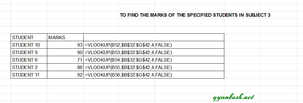
SOLVING THE #N/A PROBLEM IN VLOOKUP
Let us make a change in the formula and put a “$” sign in front of row address and column address of the lookup range. So, the formula become
=VLOOKUP(B52,$B$32:$G$42,4,FALSE)
The change has been highlighted with a RED COLOR.
Now the range has been fixed and it’ll remain the same even if we drag our formula.
Drag the formula again after changing the formula.
CONFUSION CLARIFICATIONS
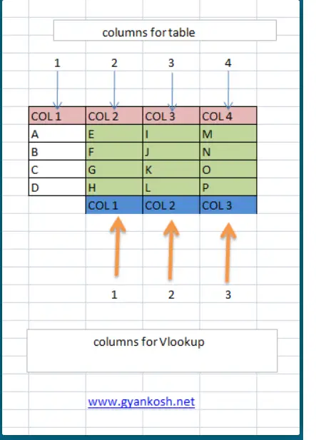
COLUMN INDEX NUMBER (INPUT NO. 3 IN VLOOKUP FORMULA)
Let us try to understand some facts about the COLUMN NUMBER in the VLOOKUP FUNCTION for GOOGLE SHEETS.
IT IS CONCERNED WITH THE LOOKUP TABLE The Range, which has been selected by us to find our desired value from, is considered a table by the GOOGLE SHEETS and its columns will be counted from the left to right.
Just put a number of the column, the value which you need to retrieve.
EXAMPLE:
Checkout the illustration given in the picture.
The Range selection area is colored in Green.
The table has four columns but for vlookup, the columns will be counted from the first column of selected range as shown by orange arrows.
This was a detailed introduction to VLOOKUP FUNCTION in google sheets .