Table of Contents
- WHAT IS A TABLE IN EXCEL?
- BUTTON LOCATION OF TABLE IN EXCEL
- STEPS TO INSERT TABLE IN EXCEL
- TABLE TOOLS
- STEPS TO USE TABLE TOOLS IN EXCEL
- EXAMPLE OF USING TABLE OPTIONS IN EXCEL
WHAT IS A TABLE IN EXCEL?
“A TABLE IS A SET OF RELATED DATA [ FIGURES(DATA) AND DETAILS] PRESENTED IN A SYSTEMATIC WAY AS ROWS AND COLUMNS”.
When we give the facts and figures in text or lengthy lines, it is always difficult to extract the information and we need to read the complete paragraph. It was when the need for a table arose. The table contains only the important figures and no theory. The benefit of tables are the ease of data crunching. We can have a look at the table and get the useful data at once.
For example,
There are 50 students in Class A, 55 in Class B, 40 in Class C
In the table, we’ll just show
Number of Students
Class A 50
Class B 55
Class C 40
It is clearly visible that the way 2, which is via the use of tabular form, the information grasping is better, clear and fast. So it is very important to be able to create tables in Excel and use them effectively.
ALTHOUGH THE GRID ITSELF ACTS AS A TABLE BUT EVEN THEN THERE ARE MANY ADDITIONAL FUNCTIONS WHICH CAN BE USED IN MANY FRUITFUL WAYS IN A TABLE.
THE ARTICLE DISCUSSES HOW TO INSERT TABLE IN EXCEL AND DIFFERENT OPTIONS AVAILABLE WITH THE USE OF TABLE.
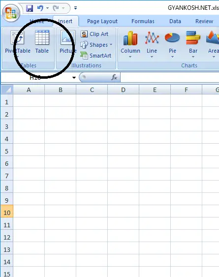
BUTTON LOCATION OF TABLE IN EXCEL
The button for inserting a table is under the INSERT TAB in the TABLES SECTION which is normally located in the left portion of the ribbon.
We can also use the KEYBOARD SHORTCUT FOR TABLE CREATION BY
“Keeping pressed the ALT KEY, press N and then T. [ ALT+N+T]”
STEPS TO INSERT TABLE IN EXCEL
- Select the data from first cell to the last cell. [The table data, including the headers]
- Click the table button.
- A small dialog box will open.
- It’ll show address of the two cells in between which you have the data. It’ll also ask if your table has headers (Headings) .If it has headers, click the checkbox. Mind it that its different from the word style of making table.
- After the data has been converted to table, we have the choice of selection from the headers which data to be displayed.
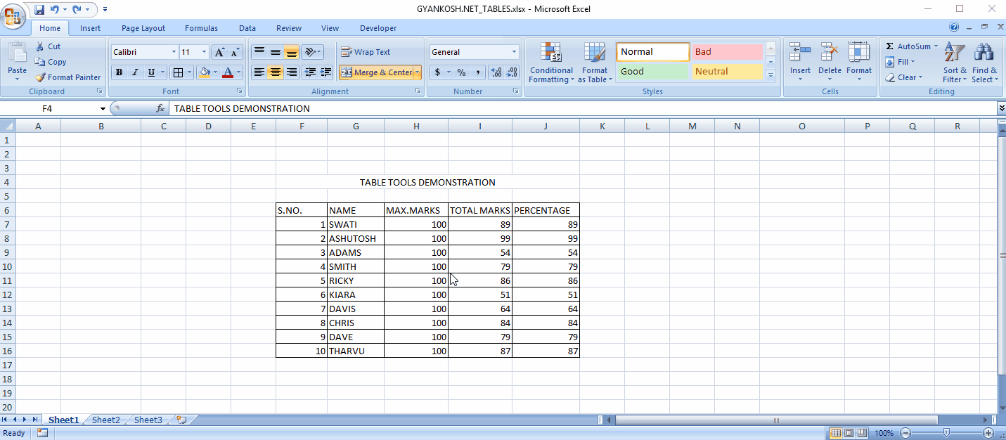
- Congrats, your table is ready as shown in the picture below.
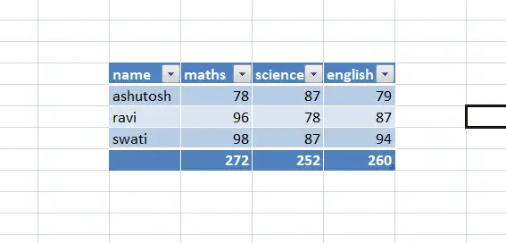
The table is shown in the picture above.
We can see that the topmost row [ header row] is having the drop-down symbols.
It helps us to choose the data which we want to show by choosing. Just press the drop-down and choose the data.
TABLE TOOLS
TABLE TOOLS ARE OPENED WHEN WE DOUBLE-CLICK OUR TABLE.
The data, which we have converted into a table now, was already in the same way in cells but now it’s a table.
After the creation of a table, Table options open with a variety of options. Look at the picture below.
A tab called DESIGN opens up when we double click our table.
Most of the options present in the DESIGN TAB for TABLES are for making the data interpretation easier.

STEPS TO USE TABLE TOOLS IN EXCEL
Table tools– Most of the options are for making the interpretation easier. Like Highlighting the columns, header row hiding, total row hiding, choosing table style, finding the duplicates, converting to range (The choice will remove the header row from the table), etc.
TABLE TOOLS:
The animated example shows the different tools present in the Table Options. [REFER TO PICTURE BELOW]
TABLE NAME: Enter the table name of your choice. It is the first option in the left portion of Table tools options.
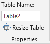
RESIZE TABLE: Click this and a small dialog box asking for the fresh range of table data would open. Choose the new data and the old table will be converted into this one.
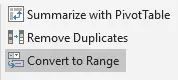
SUMMARIZE WITH PIVOT TABLE: Convert the table into PIVOT TABLE. [CLICK HERE TO KNOW PIVOT TABLES].
REMOVING DUPLICATES:
The example shows the option of removing duplicated data by choosing the column on which the check is to be applied. Excel will apply the check on the columns which are selected and remove the duplicate items.(The duplicate items will be searched only from the checked columns. Both columns should have the same duplicate value, only then this option will work.).[CLICK HERE FOR DETAILS]
CONVERT TO RANGE: The table is converted to a range. The drop-down from the header row is removed and it becomes a simple set of cells just with the colors. No TABLE OPTIONS are available after it becomes a range.

INSERT SLICER: Insert a slicer for smart filtering. [CLICK HERE TO KNOW SLICERS].
CHOOSING TABLE STYLE OPTIONS: The table style can be easily chosen from the Table Styles list as shown in the example.
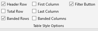
HEADER ROW: Display or remove the header row. The top row with color and filter buttons.
TOTAL ROW: Display or hide the TOTAL ROW. A row at the bottom to show the column totals.
BANDED ROW: The alternate colors for the table for better visibility.
FIRST COLUMN: Highlights the first column of the table.
LAST COLUMN: Highlights the last column of the table.
BANDED COLUMNS: Bands of colors to alternate columns, if needed.
FILTER BUTTON: Display or hide the FILTER BUTTON from the header row.
EXAMPLE OF USING TABLE OPTIONS IN EXCEL
These were the ways to create a table and use many table tools in Excel.