Table of Contents
- INTRODUCTION
- WHERE IS REMOVE DUPLICATES PRESENT IN EXCEL?
- PURPOSE OF REMOVE DUPLICATES IN EXCEL?
- WAY TO USE REMOVE DUPLICATES IN EXCEL
- FAQs
INTRODUCTION
Many times in our reports we are stuck will lengthy columns containing hundreds or thousands of rows. Sometimes these columns contain repeated rows, which are extremely hard to find manually because if we do so, it is going to be very hectic and time-consuming.
But thanks to Excel which provides us with many options to remove such repeated data easily.
In this article, we will discuss one such method.
The method is to remove the duplicated rows from the given columns.
EXCEL provides us a direct solution for the problem known as REMOVE DUPLICATES.
This option facilitates instantly removing the duplicate values from any column. The option removes all the duplicated rows and creates a new column with unique values only.
There are several options that EXCEL asks for before we execute the option. Let us find out the way to use the REMOVE DUPLICATE option in Excel.
WHERE IS REMOVE DUPLICATES PRESENT IN EXCEL?
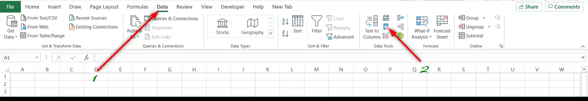
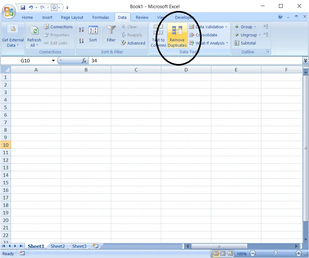
The button for REMOVING DUPLICATES can be found under the DATA TAB >DATA TOOLS as shown in the picture below.
PURPOSE OF REMOVE DUPLICATES IN EXCEL?
REMOVE DUPLICATES helps us to remove the duplicate values from a set of data.
This is important when we need the unique values only which are not repeated at all.
REMOVE DUPLICATES remove the repetition of the values in a particular column or more than one column.
Its application is very handy in keeping the unique values and removing the repetitive values.
WAY TO USE REMOVE DUPLICATES IN EXCEL
- Select the column or a range, from which you want to remove the duplicate values.
- Go to DATA TAB > Click the button, remove duplicate or click ALT+A+M.
- A dialog box as shown in picture will open.
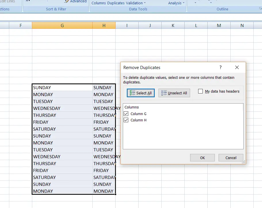
- Select the columns for the checking of duplicate values and click OK.
- All the values with the repeated values will be removed and the unique values will be left.
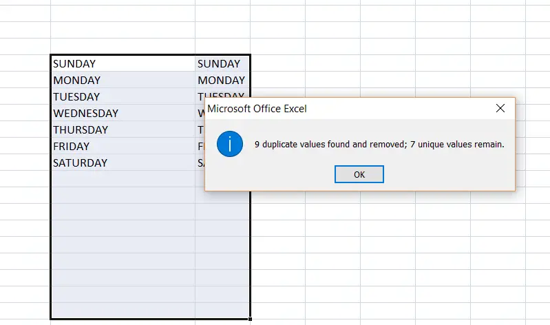
The following picture shows the result.
A small dialog box shows the number of duplicate values found and the remaining unique values.
OUTPUT
The duplicate values from each column have been removed as desired. The data is left without any repeated value.
FAQs
SHOULD I SELECT ALL THE COLUMNS OR ANY ONE COLUMN OF MY DATA FOR REMOVING DUPLICATES?
Normally One Row represents One complete set of information. So select all the data including all columns so that the operation done on one cell is equally applied to other columns also to keep the integrity of your data.
WHICH COLUMN SHOULD BE SELECTED FOR THE DUPLICATE REMOVAL?
After selecting all the data, select the column or columns which need to be scanned for duplicate removal.
For Example, if we have the following data.
| ROW NO. | A | B | C |
| 1 | HI | EVERY | ONE |
| 2 | ONE | HI | EVERY |
| 3 | EVERY | HI | ONE |
| 4 | ONE | HI | EVERY |
| 5 | EVERY | EVERY | ONE |
SELECTION: If we want that all the data to be integrated, i.e. Row no. 3 should contain the correct data only, we need to select all the data before applying the REMOVE DUPLICATES option.
CHOOSING THE REMOVE DUPLICATES COLUMNS
For this, if we select COLUMN A, EXCEL will search the duplicates in column A and drop all the other occurrences after the first one.
So, the result will display only rows 1 , 2 and 3 because Row no. 4 and 5 are repeated as per column A.
Similarly, if we select COLUMN B and COLUMN C, Row no. only row 1,2, and row no. 1,2 will remain while omitting the other rows respectively.
If we select all three COLUMNS I.e. A, B, and Crow no. 1,2,3 and 5 will remain as row no. 4 is the copy of row no. 2.
Concluding all the discussion and results, it can be simply understood that all the columns which are included in the comparison need to exact same copy of the other, only then it’ll be treated as a duplicate.
It means if we are removing the duplicates on the basis of COLUMN A and COLUMN B then the values of both the rows should have the same values at COLUMN A and COLUMN B.