INTRODUCTION
AVEDEV FUNCTION comes under the STATISTICAL FUNCTIONS category in Excel.
AVEDEV or AVERAGE DEVIATION function , as the name suggests, finds out the average of the ABSOLUTE (POSITIVE OF NEGATIVE, THE DEVIATION WILL BE TAKEN AS A VALUE I.E. POSITIVE) deviations from the mean of the data set.
Average , as we know is calculated by dividing the total sum of all the values by the number of items.
This function, first of all finds out the mean of the data.
The mean or average of the data is found.
After finding the mean, individual points are subtracted from the mean. After this, the average of the individual deviations is found.
PURPOSE OF PROPER FUNCTION IN EXCEL
AVEDEV FUNCTION returns the AVERAGE OF THE ABSOLUTE DEVIATIONS FROM THE MEAN of the data set.
PREREQUISITES TO LEARN AVEDEV FUNCTION
THERE ARE A FEW PREREQUISITES WHICH WILL ENABLE YOU TO UNDERSTAND THIS FUNCTION IN A BETTER WAY.
- Basic understanding of how to use a formula or function.
- Basic understanding of rows and columns in Excel.
- Some information about the STATISTICAL terms is an advantage for the use of such formulas.
- Of course, Excel software.
Helpful links for the prerequisites mentioned aboveWhat Excel does? How to use formula in Excel?
SYNTAX: AVEDEV FUNCTION
The Syntax for the function is
=AVEDEV(NUMBER1, NUMBER2…)
NUMBER The data set numbers.
At least one number is needed and at most 255 numbers can be entered.
EXAMPLE:AVEDEV FUNCTION IN EXCEL
DATA SAMPLE
Let us take an example of 8 numbers and analyze them with the formula and manually.Let the numbers be 2 3 4 5 3 2 7 5The examples are always taken as simple and small so that the new comers can easily understand. But the truth is, whatever be the size of the data, the analysis would remain the same so never worry about this.
STEPS TO USE AVEDEV FUNCTION-EXAMPLE
MANUAL CALCULATION.
The calculation is very simple.
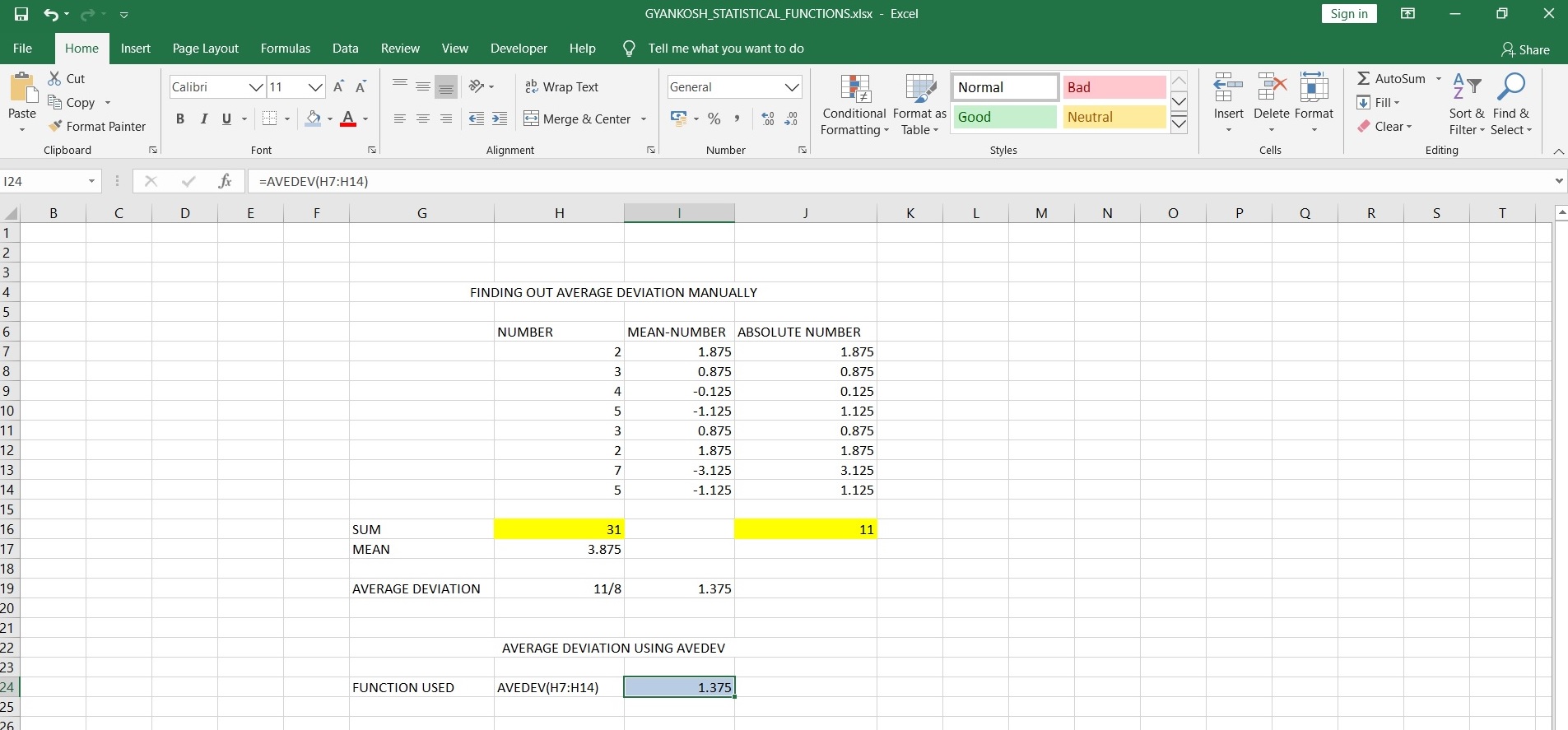
The data is put in from H7 TO H14. The total of the values is 31 which is further divided by the number of items
which is 8. 31/8 comes out to be 3.875 which is the mean of the data.
In next column, the number is subtracted from the mean to find out the deviation from the mean but it should be kept in mind that deviations can be positive or negative but in this function we are talking about absolute deviations. So in the next column we made all the values absolute by using the function ABS.
The total of the deviation is 11 which is divided by 8 .
The result, absolute average deviation of the given dataset when calculated manually comes out to be
1.375.
now let us calculate the same using the formula.
The function is directly used in cell I24.
=AVEDEV(H7:H14)
The numbers can be input one by one or a full range as shown above.
The result comes out directly to be 1.375 which proves our manual calculation also.
So its clear from the above discussion how easy the life becomes if we have handy formulas.
GENERALIZED STEPS TO USE AVEDEV function
STEPS:
1. PLACE THE CURSOR IN THE CELL WHERE WE NEED THE OUTPUT OR ANSWER.
2. TYPE IN THE CELL “=AVEDEV(RANGE OF THE DATA OR NUMBER1, NUMBER 2 …)”.
3. CLICK ENTER.
4. The result will appear.