Table of Contents
- INTRODUCTION
- PREREQUISITES TO USE SLICER IN GOOGLE SHEETS
- BUTTON LOCATION FOR SLICER
- STEPS TO CREATE A SLICER IN GOOGLE SHEETS
- EXAMPLE : CREATE A SLICER TO FILTER RAINFALL AS PER THE REQUIREMENT IN GOOGLE SHEETS
- EXAMPLE DATA:
- SOLUTION:
- USING THE SLICER IN GOOGLE SHEETS
- APPLYING MULTIPLE SLICERS
- CONCEPT FOR APPLYING MULTIPLE SLICERS
- USING MULTIPLE SLICERS
- HOW TO DELETE/REMOVE A SLICER IN GOOGLE SHEETS?
INTRODUCTION
SLICERS are a new way of filtering data in Google Sheets.
Its mostly graphical, easy to use and help us to see what is the current condition of the filtration state.
Slicers gives us the option of slicing the columns into small tables which further gives us the control of filtering the data.
The slices are something like this as shown in the picture below.
PREREQUISITES TO USE SLICER IN GOOGLE SHEETS
The SLICER can’t be used anywhere we want.
SLICER is specifically meant for tables only or the data of the graphical representations like charts and graphs . The table can be a SIMPLE TABLE or the PIVOT TABLE.
Here we’ll be discussing slicer with the help of normal tables only. Slicer for the PIVOT TABLE will be dealt in the PIVOT TABLE article only. So let us try to create a slicer for the table.
BUTTON LOCATION FOR SLICER
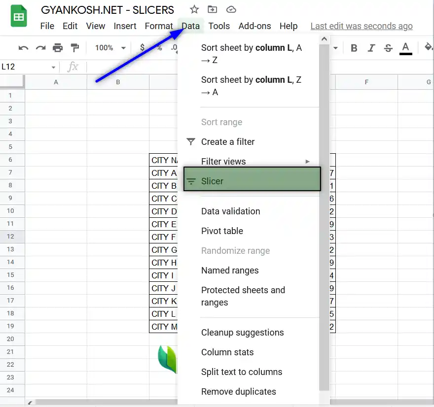
The SLICER is located under the INSERT TAB in FILTER OPTIONS. The picture below shows the button location for SLICER.
STEPS TO CREATE A SLICER IN GOOGLE SHEETS
STEPS:
- Create a table having some data so that we try our slicer on that.
- If you don’t know how to create a table.
- Go to DATA MENU > SLICERS.
- The SLICERS window, a window asking for the range and option box on the right side will open. [ Don’t worry! It is just a brief. We’ll perform each step with complete description and picture while taking an example.
- Enter the range in the SELECT A DATA RANGE box and click OK.
- Go to the right and select the column for the filtration from the SLICER OPTIONS.
- The slicer is ready.
- You can use the slicer to filter the data by putting the values to be shown or not shown as well as putting the conditions.
- The slicer is ready.
Let us try this with the help of an example.
EXAMPLE : CREATE A SLICER TO FILTER RAINFALL AS PER THE REQUIREMENT IN GOOGLE SHEETS
EXAMPLE DATA:
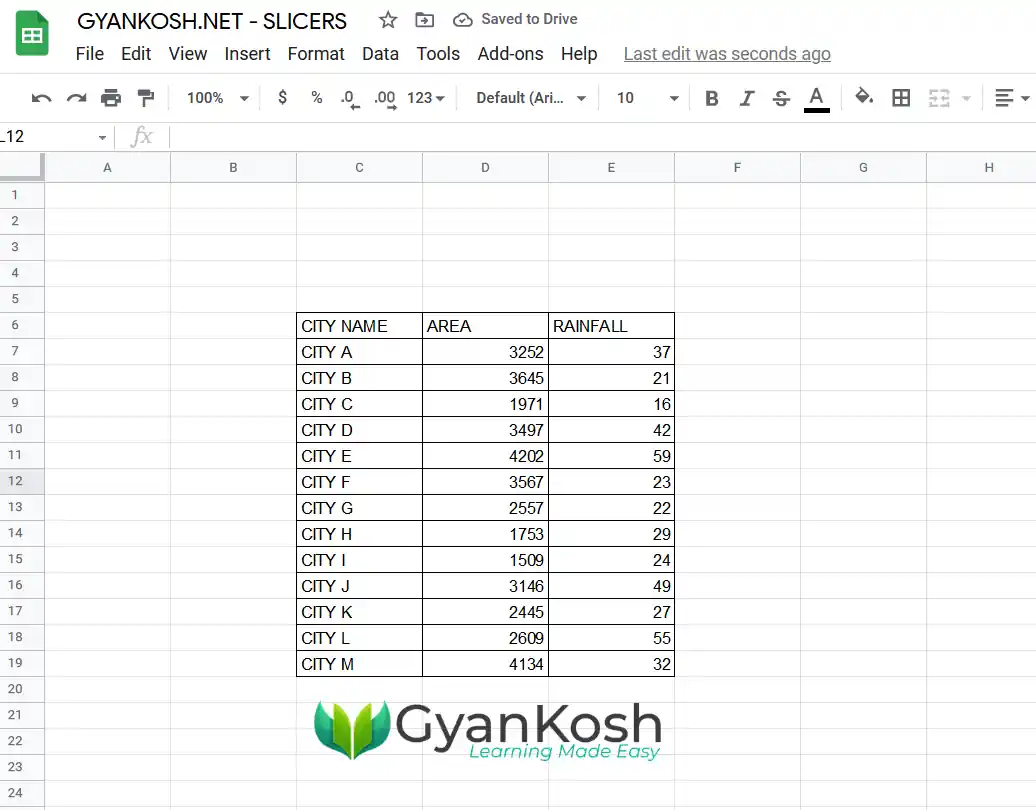
The example contains the area and rainfall of the different cities.
We’ll create a slicer to control the RAINFALL
The three columns contain the CITY NAME, AREA and RAINFALL.
The table is shown in the picture below.
NOTE: Choose those options which are the basis of filtering. Don’t choose all the options as it’ll only mess up the screen.
SOLUTION:
We can easily create a filter to control the data on the basis of the rainfall values.
FOLLOW THE STEPS TO CREATE A SLICER
- Select the complete data range including the headers. [ We can do this later too as per the previous discussed steps.]
- Go to DATA MENU and choose SLICER.
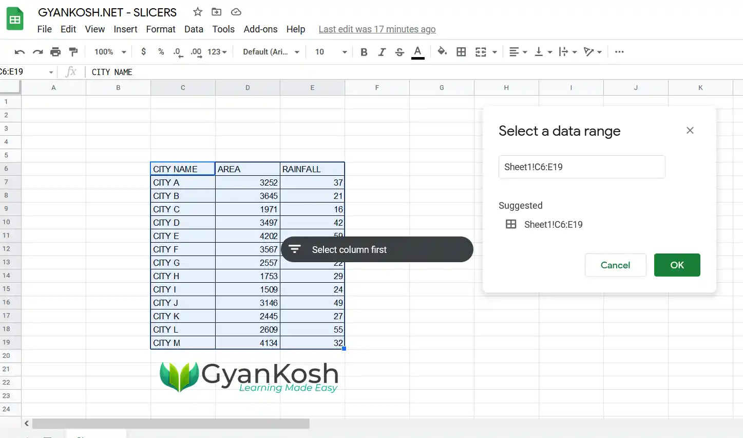
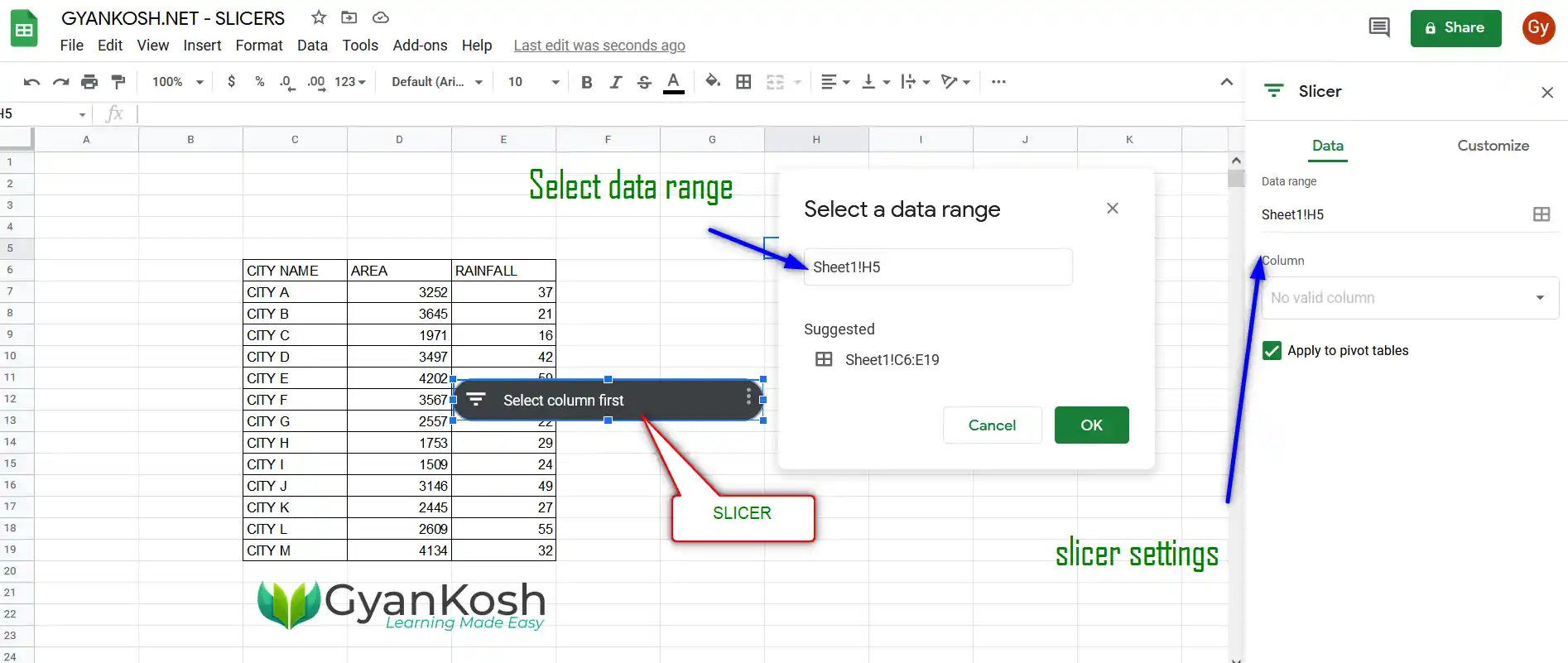
- The following options will appear.
SELECT A DATA RANGE: For selecting the data in subject i.e. the range containing the data including the headers. This option won’t appear if you have selected the data first and then opted for SLICER.
SLICER BAR: The slicer will be controlled from a small bar which is currently showing SELECT COLUMN FIRST.
SLICER OPTIONS on the right window: It contains all the options required to customize and control SLICER.
The following picture shows the discussed options.
;
- Enter the range as C6:E19 in the SELECT A DATA RANGE. [ If you already selected the data before opting for slicer, this window won’t open up and the selected data will be taken automatically.]
- After choosing the data range, go to the SLICER OPTIONS on the right portion of the screen.
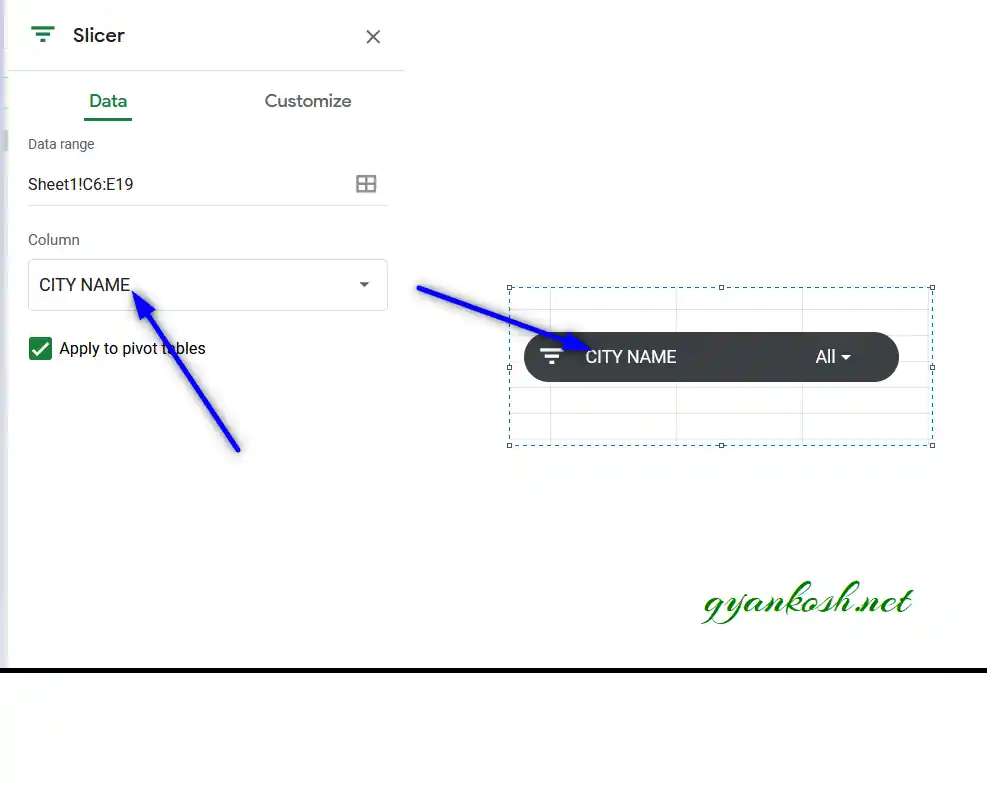
- Go to the COLUMN DROP DOWN and choose the column on the basis of which you want to filter the data.
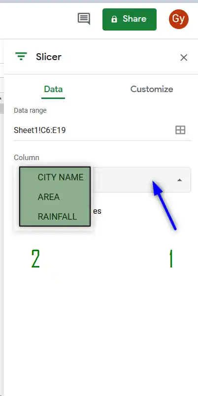
As soon as we choose the column name, it’ll start appearing over the SLICER CONTROLLING BAR as shown in the picture below.
For the example, if we choose CITY NAME as the column, it’ll reflect on the SLICER too.
For our example, we’ll be taking the slicer column as RAINFALL. So change the column name and the slicer will change the label as RAINFALL.
The slicer has been deployed. Now we’ll see how to use them.
USING THE SLICER IN GOOGLE SHEETS
After we have successfully created a SLICER, it is really easy to use one.
FOLLOW THE STEPS TO USE THE SLICER
- The slicer will show the label which will be one of the COLUMN HEADINGS of the table showing the data.
- Click the drop down showing ALL.
- Choose FILTER BY CONDITION and choose the condition.
- For our example we chose the CITIES having the rainfall greater than 50.
- Go to FILTER BY CONDITION.
- Choose GREATER THAN
- Enter 50 in the field.
- Scroll down and click OK.
- The table will show only the cities having the rainfalls greater than 50.
The following animation shows the complete process.
In this way, we can create and use a slicer in Google Sheets.
We can also put multiple Slicers on the same data. Let us try to apply two slicers managing the AREA and RAINFALL on the same data.
APPLYING MULTIPLE SLICERS
If we want to apply more than one slicer to the same data, we can do that quite easily.
ONE SLICER WILL CONTROL/FILTER THE DATA ON ONE CHOSEN CRITERION. IT MEANS WE'LL NEED TWO SLICERS IF WE WANT TO FILTER THE DATA ON TWO SEPARATE CONDITIONS.
CONCEPT FOR APPLYING MULTIPLE SLICERS
The slicers can easily be applied on the same data.
The process is to simply create two slicers in the same way we apply a single slicer one after the other.
The controlling COLUMNS can be different and both will work separately.
FOLLOW THE STEPS TO APPLY THE MULTIPLE SLICERS ON THE SAME DATA
Apply the slicer as we discussed in the previous sections.
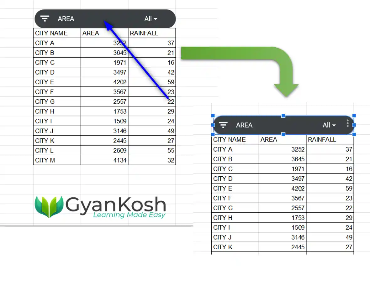
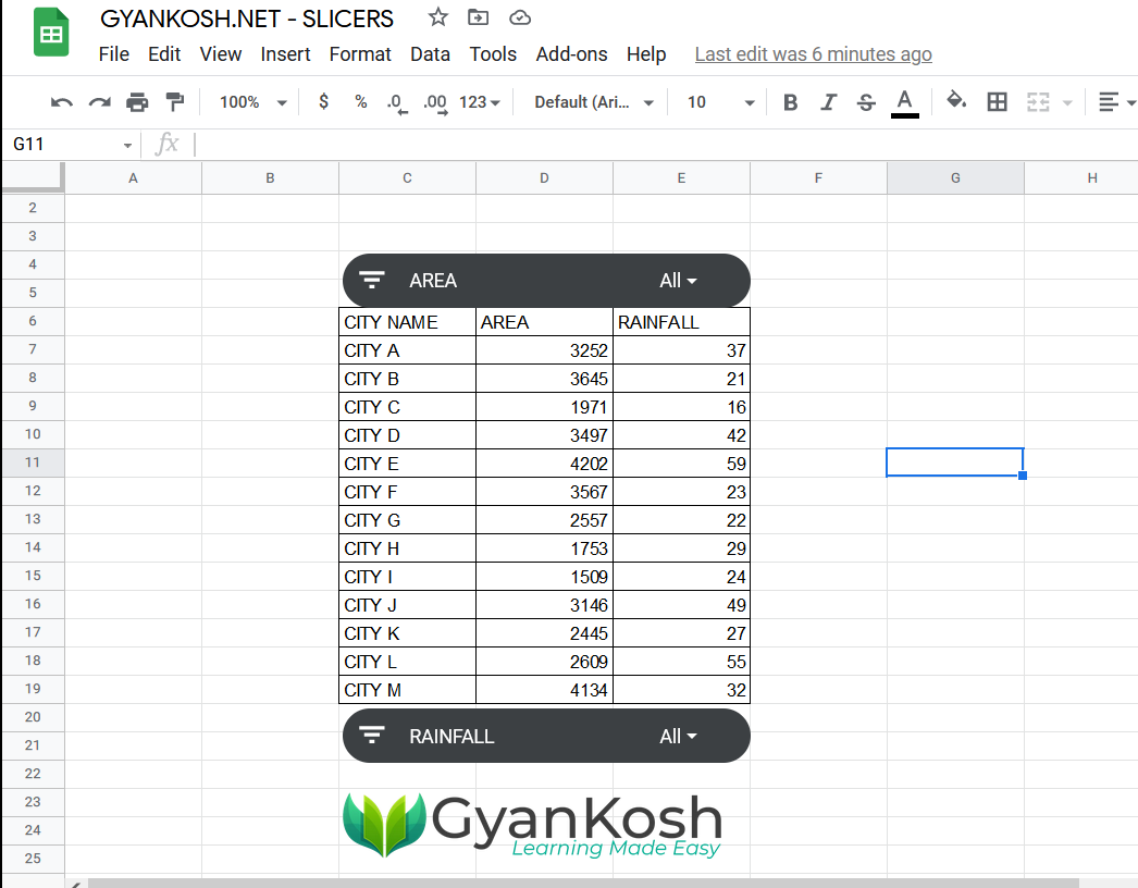
Repeat all the steps but choose the COLUMN as AREA.
The two slicers will be created as shown in the picture below.
USING MULTIPLE SLICERS
The multiple slicers are used in the exact same way the single slicer is used.
THE MULTIPLE SLICERS CREATE THE AND CONDITION ON THE DATA.
AND CONDITION IS THE ONE WHICH IS TRUE ONLY WHEN BOTH THE CONDITIONS AGREE.
IN THE EXAMPLE, THE TWO CONDITIONS I.E. AREA AND RAINFALL ARE TAKEN INTO ACCOUNT.
THE RESULT WILL SHOW THE DATA WHICH WILL COMPLY BOTH THE CONDITIONS CHOSEN FROM THE SLICER 1 AND SLICER 2.
FOLLOW THE STEPS TO USE MULTIPLE SLICERS IN GOOGLE SHEETS
- Click dropdown from the AREA SLICER and choose FILTER BY CONDITION and choose the condition.
- For our example we choose the AREA GREATER THAN 2000 and click OK.
- The data will remove all the data which contain the AREA less than or equal to 2000.
- Now, go to RAINFALL SLICER and choose FILTER BY CONDITION.
- Choose condition as IS BETWEEN and enter the lower and higher values as 20 and 25.
- It’ll remove all the rows from the remaining data which satisfies the rainfall condition.
- The following animation shows all the described process.
HOW TO DELETE/REMOVE A SLICER IN GOOGLE SHEETS?
The process is quite simple.
FOLLOW THE STEPS TO DELETE A SLICER
- Select the slicer by clicking it.
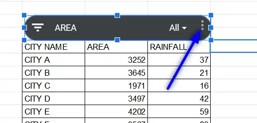
- After selecting the slicer, click on the three dots at the right portion for showing more options.
- As we click the THREE DOTS, more options will appear.
- Click on DELETE SLICER.
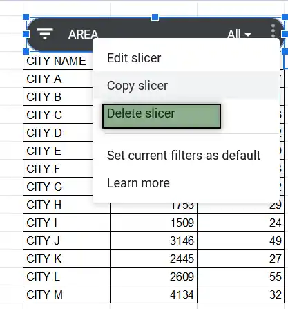
- The slicer will be deleted or removed.
- The condition on the data, if selected will be removed and all the data will be visible.
