Table of Contents
- INTRODUCTION
- WHAT IS A PIVOT TABLE IN GOOGLE SHEETS?
- WHERE DO I FIND PIVOT TABLE OPTION IN GOOGLE SHEETS?
- WHAT ARE THE USES OF PIVOT TABLE IN GOOGLE SHEETS?
- STEPS TO CREATE PIVOT TABLE IN GOOGLE SHEETS
- HOW TO ADD FIELDS TO ROWS, COLUMNS, VALUES OR FILTERS IN GOOGLE SHEETS
- EXAMPLE 1 :HOW TO CALCULATE THE TOTAL SALES PER DAY
- EXAMPLE 2: HOW TO CALCULATE THE AVERAGE SALES PER DAY
INTRODUCTION
In this article, we would learn to create a pivot table in google sheets from the scratch and use it in different ways.
PIVOT TABLE is a well-known feature of GOOGLE SHEETS that everybody of us might have heard of. But many of us have never used them.
PIVOT TABLE is a dynamic table that we can create in GOOGLE SHEETS. We called it dynamic as we can transform it within seconds. The original data remains the same.
We know that whatever is hinged to a pivot, can rotate here and there, and so is the name given to these tables.
PIVOT Table is a very powerful tool to summarize, analyze explore the data in very simple steps. It’s very important to learn the use of pivot tables in Google Sheets if we want to master it. Pivot tables give us the facility to put different simple operations on selected data in seconds.
WHAT IS A PIVOT TABLE IN GOOGLE SHEETS?
A pivot table is a simple table but can be changed dynamically.
We know that whatever is hinged to a pivot, can rotate here and there, so is the name given to these tables as we can change the rows and columns in the way we want within the seconds and can derive the different results.
It means, it is a table but gives us the total flexibility to play with the data.
For Example, We put all the fields in a pool and we can choose any field to be put in Rows or Columns.
So, we can simply shift the fields from this pool from rows to columns or columns to rows within a second.
We can also change the result like sum, average, or any other operation within seconds.
We can simply put any data from row to column or column to row within the seconds.
WHERE DO I FIND PIVOT TABLE OPTION IN GOOGLE SHEETS?
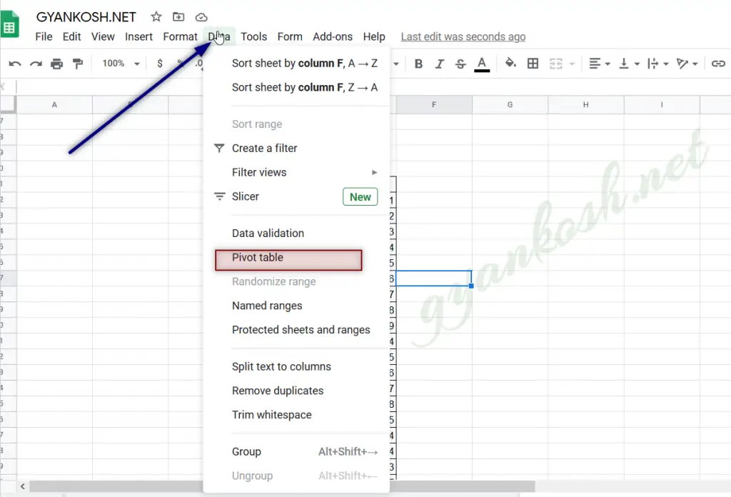
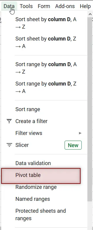
Let us find out where we can find out the option for creating a PIVOT CHART in GOOGLE SHEETS.
Look at the picture below.
The PIVOT TABLE option is found under the DATA MENU>PIVOT TABLE option.
WHAT ARE THE USES OF PIVOT TABLE IN GOOGLE SHEETS?
Let us discuss the benefits of using pivot tables and their uses in Google Sheets.
Pivot tables are used when
- we need to analyze large data in a short notice.
- we need to total, summarize, category wise, sub category wise, perform different calculations like sum, average, or any custom calculation etc.
- A collapsible presentation, which we can twist and present in our own way within a few seconds.
- Play with rows and columns and create different reports.
- we need to filter, group, sort and conditionally format the data.
STEPS TO CREATE PIVOT TABLE IN GOOGLE SHEETS
Let us understand the steps to create a pivot table using an example.
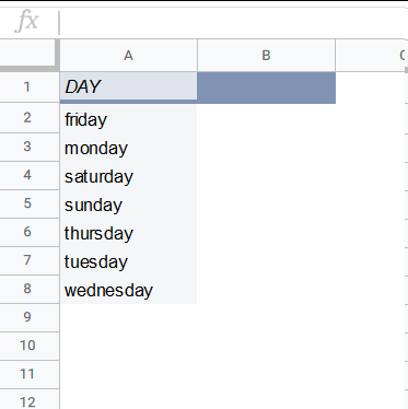
DATA SAMPLE:
The table and picture below show the Sales of Cars for every day of a month. [ Only a portion is available].
We will create a PIVOT TABLE for the given data and see what kind of different operations we can perform on this data within seconds.
| DAY | SALES |
| sunday | 1 |
| monday | 2 |
| tuesday | 3 |
| wednesday | 4 |
| thursday | 5 |
| friday | 6 |
| saturday | 7 |
| sunday | 8 |
| monday | 9 |
| tuesday | 4 |
| wednesday | 5 |
| thursday | 6 |
| friday | 7 |
| saturday | 8 |
| sunday | 5 |
| monday | 4 |
| tuesday | 4 |
| wednesday | 3 |
| thursday | 7 |
| friday | 9 |
| saturday | 7 |
| sunday | 3 |

STEPS TO CREATE A PIVOT TABLE:
- Select the data including headers, go to DATA MENU and choose PIVOT TABLE BUTTON.
- Click PIVOT TABLE BUTTON. A dialog box will open as shown in the following pic.
- As we have already selected the table, the range would show up automatically, otherwise, we can put it manually or by selecting the table.
- If we haven’t selected the range, we can put it manually too. The standard format will be ‘SHEET NAME’!RANGE
- Choose the location for the pivot tables. It can be on a NEW WORKSHEET or EXISTING SHEET. If the existing worksheet, we need to tell the starting cell location. [If no specific requirement is there, always choose to create a PIVOT TABLE on NEW SHEET ]
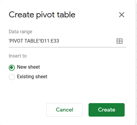
- CLICK CREATE.
- It’ll take us to the new sheet [If opted for new sheet or the cell location in the same sheet where we chose to create the pivot table. ]
- Our PIVOT TABLE is ready but it hasn’t taken its shape yet.
* We will all the options in detail in the next portion of the article.
CHOOSING DIFFERENT OPTIONS TO CREATE PIVOT TABLE:
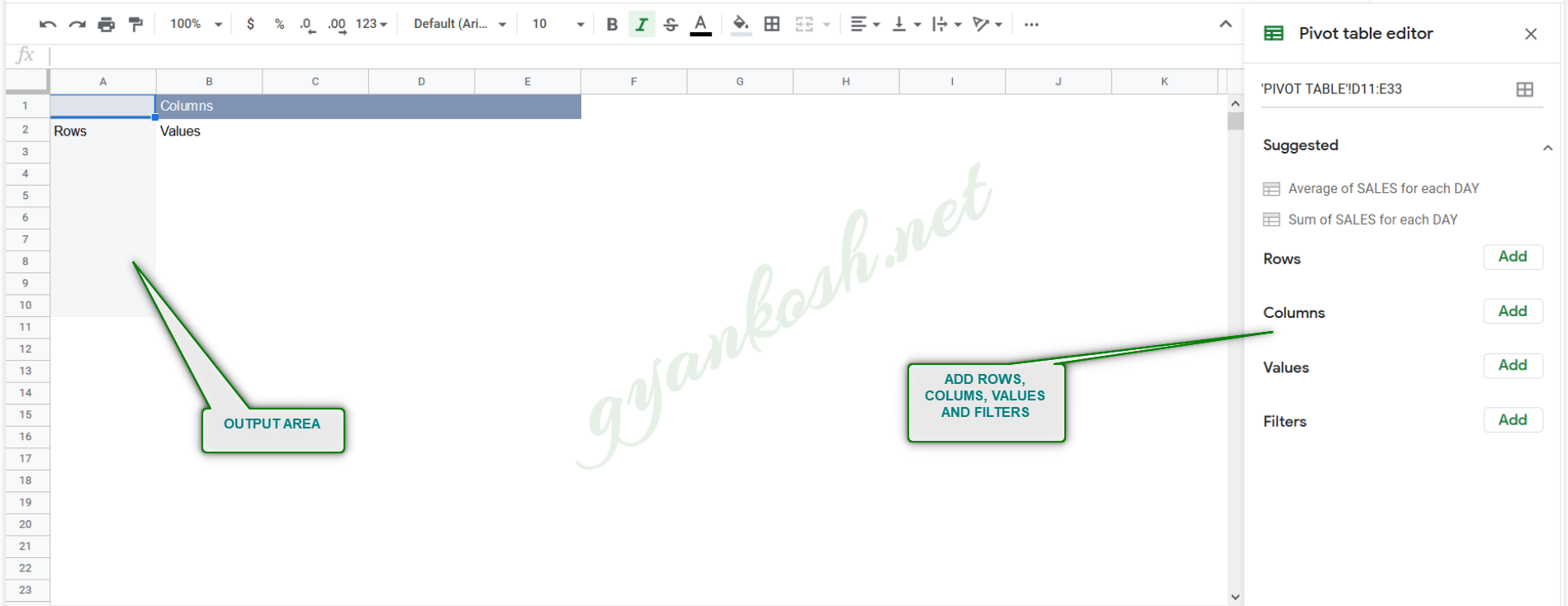
In the picture above we can see that an empty structure of the PIVOT TABLE has been created.
On the RIGHT SIDE of the screen are the different options from where we can choose the different columns which we want to put in ROWS , COLUMNS , VALUES or FILTER
HOW TO ADD FIELDS TO ROWS, COLUMNS, VALUES OR FILTERS IN GOOGLE SHEETS
LET US FIRST UNDERSTAND THE DIFFERENT OPTIONS IN WHICH WE CAN PUT OUR FIELDS
Click all the fields available on the right box named PIVOT TABLE FIELD LIST.
Now let us understand the different areas of the PIVOT TABLE SHEET.
Pivot table screen has the following area. LOOK AT THE PICTURE BELOW FOR BETTER UNDERSTANDING.
Let us discuss all the areas one by one.
THE LEFT AREA SHOWS THE OUTPUT OF THE PIVOT TABLES AS PER THE SELECTION MADE IN THE EDITING DROP DOWNS ON THE RIGHT.ROWS :
The fields which we need as rows. Click the ADD and a list will appear as drop down of all the columns.
Choose the field which you want to show as ROW. For this example we chose the DAY column so that we can check the day wise sale.
COLUMNS: This field will contain the columns of our pivot tables. For examples, if we need the values, we need to select values from the dropdown list there. Click ADD to get the list of available fields and click to choose.
VALUES: The output values area. We need to specify the operation which must be applied on our data so that we get the output. We can select many operations in this field which we will see in other post.We put the fields in this area which we want to calculate.
FILTERS: It is an optional area. We can create filters there to keep the data we want. We can create a filter of any of the field and choose the data according to that.
EXAMPLE 1 :HOW TO CALCULATE THE TOTAL SALES PER DAY
LET US CALCULATE THE TOTAL SALES PER DAY
FOLLOW THE STEPS TO CALCULATE THE TOTAL SALES PER DAY:
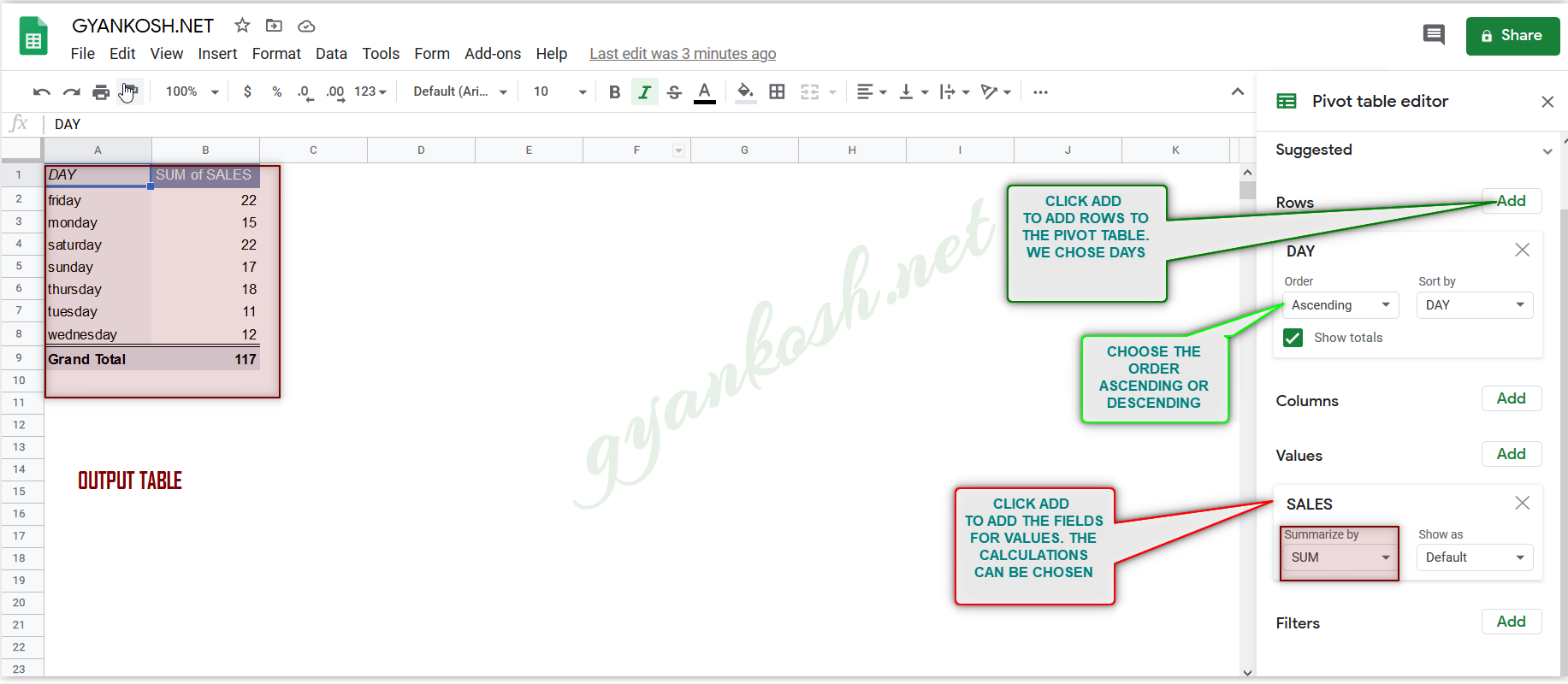
- Click ROWS>ADD.
- It’ll open a drop down showing the available fields.

- Choose DAY. It’ll list all the days in the rows under column 1. [DAY]

- Now go to VALUES .
- Click ADD, which will show the available fields in the drop down.
- Choose SALES. [ As we need sum of the sales.]
- The following screen will be seen under the VALUES.
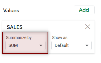
- We have SUM BY DEFAULT in the SUMMARIZE BY drop down which is marked in the picture above.
- If the selection is not SUM, choose it.
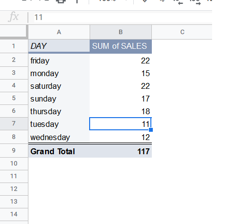
- The Table will show the TOTAL SALES DAY WISE.
LOOK AT THE PICTURE BELOW FOR BETTER UNDERSTANDING.
EXAMPLE 2: HOW TO CALCULATE THE AVERAGE SALES PER DAY
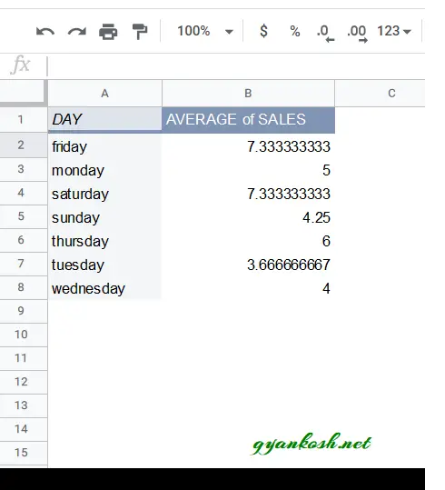
LET US CALCULATE THE AVERAGE SALES ON A PARTICULAR DAY IN THE GIVEN DATA
FOLLOW THE STEPS TO CALCULATE THE AVERAGE SALES PER DAY:
- Click ROWS>ADD.
- It’ll open a drop down showing the available fields.
- Choose DAY. It’ll list all the days in the rows under column 1. [DAY]
- Now go to VALUES .
- Click ADD, which will show the available fields in the drop down.
- Choose SALES. [ As we need sum of the sales.]
- The following screen will be seen under the VALUES.

- We have SUM BY DEFAULT in the SUMMARIZE BY drop down which is marked in the picture above.
- CLICK the SUMMARIZE BY drop down and choose AVERAGE.
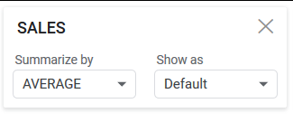
- The Table will show the TOTAL AVERAGE SALES PER DAY.
LOOK AT THE PICTURE BELOW FOR BETTER UNDERSTANDING.