WHAT IS A TABLE IN GOOGLE SHEETS?
“A TABLE IS A SET OF RELATED DATA [ FIGURES(DATA) AND DETAILS] PRESENTED IN A SYSTEMATIC WAY AS ROWS AND COLUMNS”.
When we give the facts and figures in text or lengthy lines, it is always difficult to extract the information and we need to read the complete paragraph. It was when the need of table arose. The table contains only the important figures and no theory. The benefit of tables are the ease of data crunching. We can have a look at the table and get the useful data at once.
For example,
There are 50 students in Class A , 55 in Class B, 40 in Class C
In the table , we’ll just show
Number of Students
Class A 50
Class B 55
Class C 40
It is clearly visible that the way 2, which is via the use of tabular form, the information grasping is better, clear and fast. So it is very important to be able to create tables in GOOGLE SHEETS and use them effectively.
ALTHOUGH THE GRID ITSELF ACTS AS A TABLE BUT EVEN THEN THERE ARE MANY ADDITIONAL FUNCTIONS WHICH CAN BE USED IN MANY FRUITFUL WAYS IN A TABLE.
THE ARTICLE DISCUSSES HOW TO CREATE GOOGLE SHEETS.
THERE IS NO DIRECT OPTION FOR CREATING TABLE IN GOOGLE SHEETS. BUT WE CAN CREATE A TABLE BY INDIVIDUAL OPTIONS AND MAKING THEM VISUALLY IMPRESSIVE.
STEP 1: PUT THE TABLE DATA IN THE CELLS
STEPS TO ENTER THE TABULAR DATA
- The first step of creating a table is to put the data in the tabular form in the cells of google sheets.
- Enter the COLUMN HEADERS or ROW HEADERS as per the requirement.
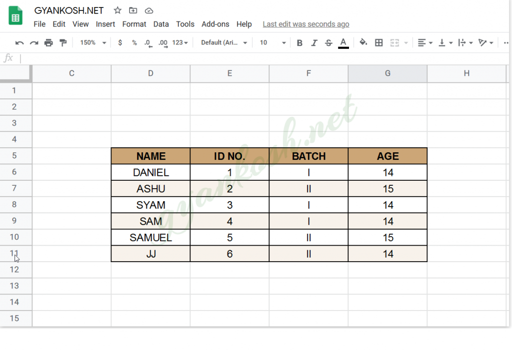
For the example, let us create a table with the student details. [ Name, Id no. Batch, Age ]
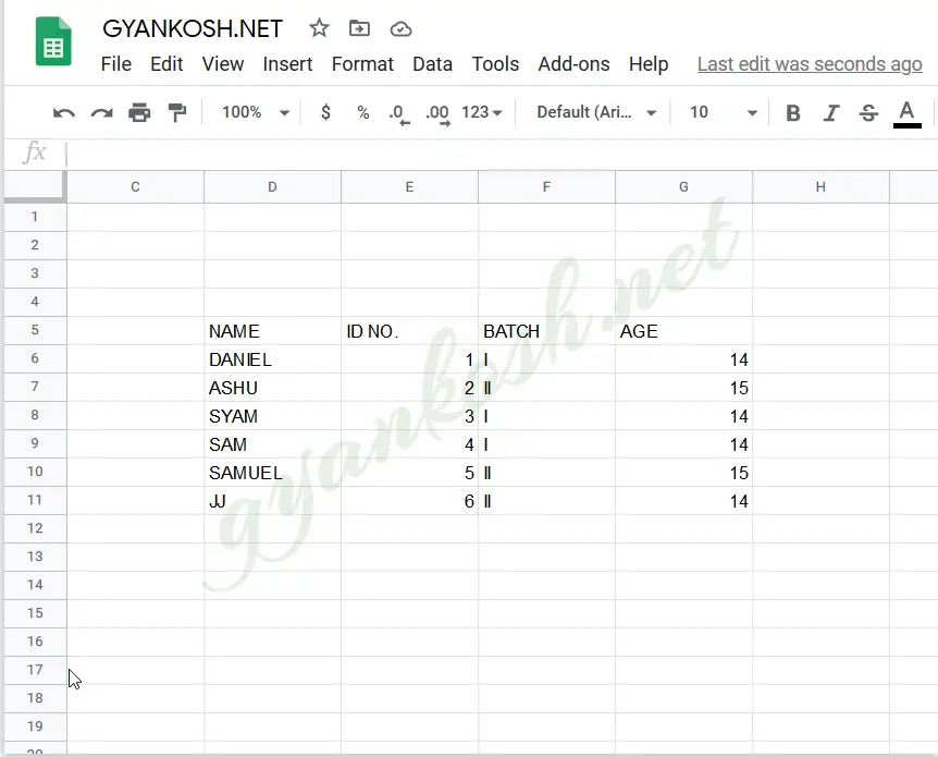
The data is shown below.
| NAME | ID NO. | BATCH | AGE |
| DANIEL | 1 | I | 14 |
| ASHU | 2 | II | 15 |
| SYAM | 3 | I | 14 |
| SAM | 4 | I | 14 |
| SAMUEL | 5 | II | 15 |
| JJ | 6 | II | 14 |
The table is shown in the picture above.
AS THERE IS NO DIRECT TABLE EDITING TOOL, WE’LL APPLY ALL THE OPERATIONS ONE BY ONE.
ALL THE OPERATIONS ARE OPTIONAL. WE CAN CHOOSE AS PER THE REQUIREMENT.
APPLY BORDER TO THE TABLE
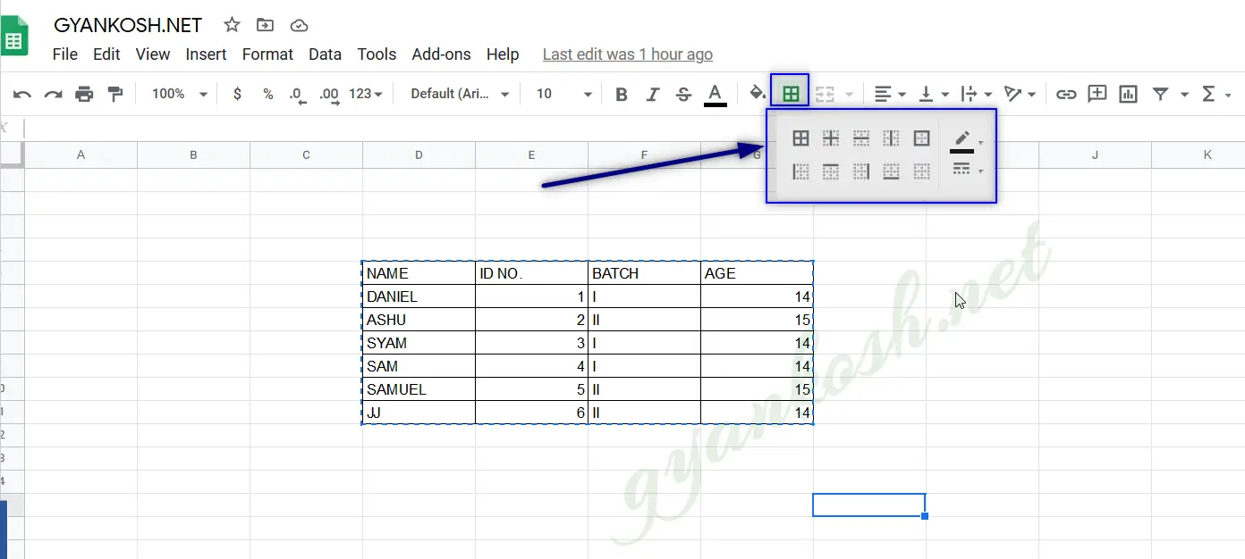
It is totally optional as per choice.If you like your table to have borders, you can easily apply them.FOLLOW THE STEPS TO APPLY THE BORDERS TO THE TABLE:
- Select the complete table including headers.
- Click the BORDERS BUTTON from the standard toolbar and choose the border as per choice.
- The reference picture is shown below.
MAKE THE HEADER OF THE TABLE BOLD
It is always advisable to make the headers bold, so that they are highlighted.
Follow the steps to make the headers bold in google sheets.
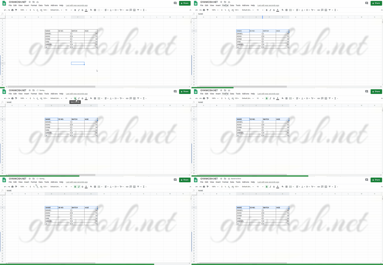
- Select the header line, and click BOLD or click FORMAT MENU and choose BOLD.
- The process is shown in the picture below.
- We can use the other formatting options too such as making the header or any other text ITALIC, or STRIKETHROUGH or UNDERLINE.
- To reverse the effect , choose the option again.
USE THE COLOR IN TABLE [ ALTERNATING COLORS ] IN GOOGLE SHEETS
To make the table still more beautiful and readable, we can put alternating colors to the table.
ALTERNATING COLORS PUT THE COLORS IN THE TABLE IN AN ALTERNATING FASHION IN WHICH ONE ROW IS FILLED WITH A COLOR AND NEXT ROW IS FILLED WITH OTHER COLOR. THE SEQUENCE IS REPEATED TILL THE END.
Follow the steps to use alternating colors in tables in google sheets.
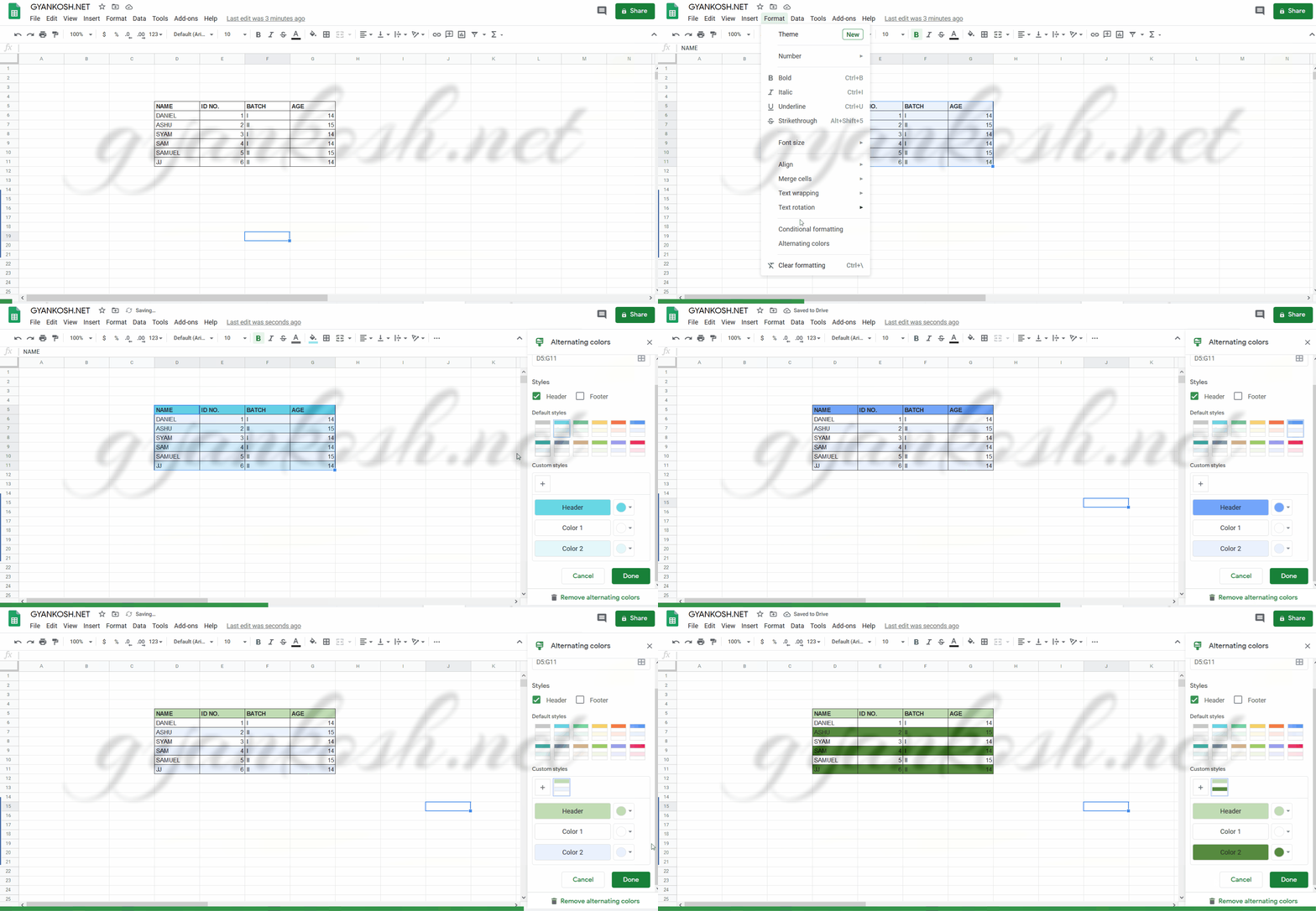
- Select the complete table which we want to color. [ We need to select all the rows in which we want the colors. The rows which are not selected won’t get any color ].
- Go to FORMAT MENU > ALTERNATING COLORS.
- As soon as we click on ALTERNATING COLORS, the table will be colored by the default colors.
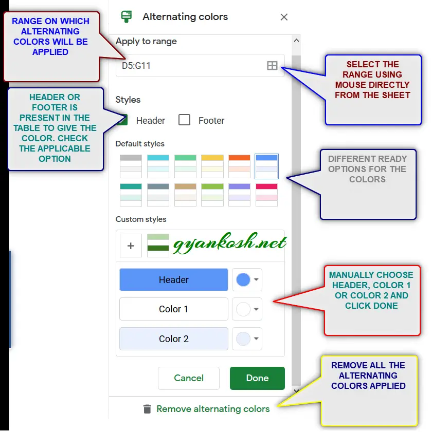
- An ALTERNATING COLORS option box will open on the right. We can choose many options from there which are discussed further in the article.
- The following picture shows the process of applying ALTERNATING COLORS and choosing the custom colors for the header, first row and second row.
After applying all the above mentioned procedures, our final table is ready.The final table looks like the one shown below.
REMOVE THE ALTERNATING COLORS FROM THE TABLE IN GOOGLE SHEETS
After the table is created, there can be the situations when we want to
-Provide custom colors to our table
-Apply the FOOTER also.
-Remove the Alternating colors.
For these problems, let us understand the use of various options provided in ALTERNATING COLORS in GOOGLE SHEETS.
THE DIFFERENT OPTIONS ARE:
APPLY TO RANGE:
The range of the cells which we have chosen for the alternating colors.
STYLES:
Select HEADER or FOOTER or both.
If only HEADER is selected, Header will be given a dark shade to highlight it.
Same with the FOOTER OPTION.
It is used to highlight the total row in the footer or any other situation like that.
DEFAULT STYLES: Ready styles from which we can choose any.
CUSTOM STYLES: Choose the HEADER, COLOR 1, COLOR 2 and FOOTER [OPTIONAL] color by manual choice.
REMOVE ALTERNATING COLORS: Remove all the colors.
In this article, we learnt about creating the tables in google sheets, making the text bold, give alternating colors to the table and other formatting options.
