Table of Contents
- INTRODUCTION
- PURPOSE OF INDEX FUCTION IN GOOGLE SHEETS
- PREREQUISITES TO LEARN INDEX
- SYNTAX: INDEX FUNCTION
- EXAMPLE 1:RETRIEVE A VALUE FROM THE TABLE USING INDEX FUNCTION
- EXAMPLE 2: RETRIEVE A COMPLETE ROW USING INDEX FUNCTION IN GOOGLE SHEETS
- EXAMPLE 3: RETRIEVE A COMPLETE COLUMN USING INDEX FUNCTION IN GOOGLE SHEETS
- CONFUSION CLARIFICATIONS
INTRODUCTION
INDEX FUNCTION comes under the LOOKUP AND REFERENCE group of functions in GOOGLE SHEETS.
INDEX FUNCTION returns the value of a cell or array in a specified relative location given by row no. and column no. in a selected range.
Relative position is the position with respect to the select LOOKUP_RANGE.
e.g.
We have five COLORS and five CODES and we need to find out a value on a particular position.So we can use INDEX function for this scenario and it’ll find out the item to be searched at a particular position.Suppose there is a table of 4 columns and 4 rows. If we want to search that what element is present at row no. 3 and column no. 4, we’ll take help of INDEX FUNCTION.
PURPOSE OF INDEX FUCTION IN GOOGLE SHEETS
INDEX FUNCTION LOOKS UP A VALUE AT A SPECIFIC LOCATION WHICH IS MENTIONED BY RELATIVE ROW NO. AND RELATIVE COLUMN NO. IN A SELECTED LOOKUP TABLE OR RANGE.
Index function in conjunction with the other functions like MATCH FUNCTION creates a very powerful duo for looking up the values in the given data.
In addition to this index function is used at a number of places for searching out the practical solutions.
PREREQUISITES TO LEARN INDEX
THERE ARE A FEW PREREQUISITES WHICH WILL ENABLE YOU TO UNDERSTAND THIS FUNCTION IN A BETTER WAY.
- Basic understanding of how to use a formula or function.
- Easier to understand if user already knows how to use VLOOKUP.
- Basic understanding of rows and columns in Google Sheets.
- Of course, google account for logging in GOOGLE SHEETS.
Helpful links for the prerequisites mentioned above
What Excel does? How to use formula in Excel?
SYNTAX: INDEX FUNCTION
The syntax ( the way how formula is phrased for GOOGLE SHEETS) of INDEX FUNCTION is
=INDEX(REFERENCE/REFERENCES IN WHICH THE VALUE WILL BE SEARCHED FOR , RELATIVE ROW NUMBER , RELATIVE COLUMN NUMBER)
REFERENCE/REFERENCES IN WHICH THE VALUE WILL BE SEARCHED FOR The table or range selected for the look up. It can be a single row or single column too.
RELATIVE ROW NUMBER ROW , FROM WHICH THE DATA WILL BE PICKED UP
RELATIVE COLUMN NUMBER COLUMN NUMBER, FROM WHICH THE DATA WILL BE PICKED UP.
NOTE: Either of the ROW NO. OR COLUMN NO. is optional but at least one should be present.
EXAMPLE 1:RETRIEVE A VALUE FROM THE TABLE USING INDEX FUNCTION
DATA SAMPLE
We’ll consider only Table A for this example.
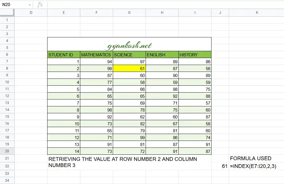
Table A have the marks of 8 students with STUDENT IDs in different subjects. We’ll find the value at row no. 2 and column no. 3 in the table.
STEPS TO SOLVE
1. Enter the following formula in any cell , where you want the result as =INDEX(E7:I14,2,3)
2. The result will appear as 89
EXPLANATION : EXAMPLE 1
The formula used for the solution is =INDEX(E7:I14,2,3)
The first argument E7:I14 is the table which we’ll consider.
Second argument is the row number which we want.
And third argument is the column number which we want.
As its clear from visual inspection the item at index 2,3 is 89 so the formula gave us the correct result.
KINDLY DON’T FORGET TO GO THROUGH THE CLARIFICATION SECTION AT THE END.
EXAMPLE 2: RETRIEVE A COMPLETE ROW USING INDEX FUNCTION IN GOOGLE SHEETS
DATA SAMPLE
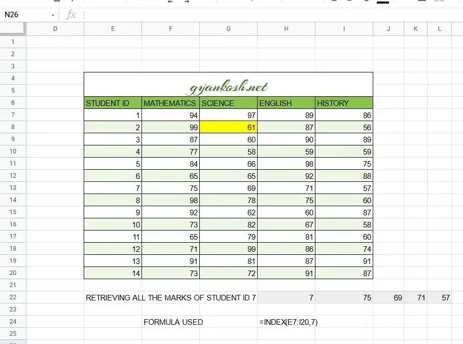
We’ll consider the same data and retrieve a complete row from the table using Index function.
Let us try to retrieve all the marks of the student with STUDENT ID 7.
STEPS TO SOLVE [EXAMPLE 2]
- Put the following formula in the cell where you want the result
- =INDEX(E7:I20,7)
- Press ENTER.
- The result will appear.
*Take care that the row is empty otherwise GOOGLE SHEETS won’t let you get the result if the result is overlapping the cells already containing the data.
EXPLANATION [EXAMPLE 2]
- The formula used is =INDEX(E7:I20,7)
- We have used only two parameters in this syntax.
- The first parameter is the REFERENCE TO THE TABLE.
- The second parameter is the ROW NUMBER 7 which is the detail of the student with ID 7.
- The result will appear.
EXAMPLE 3: RETRIEVE A COMPLETE COLUMN USING INDEX FUNCTION IN GOOGLE SHEETS
DATA SAMPLE
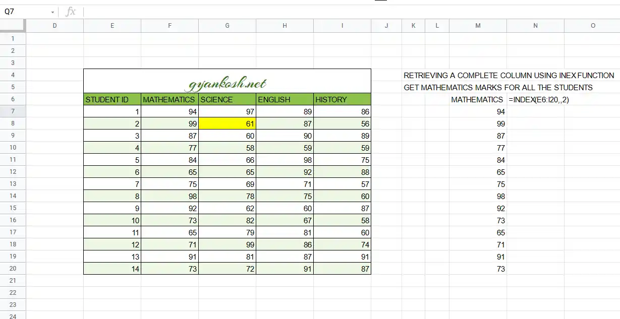
We’ll consider the same data and retrieve a complete COLUMN from the table using Index function.
Let us try to retrieve all the marks in MATHEMATICS SUBJECT.
STEPS TO SOLVE [EXAMPLE 3]
- Put the following formula in the cell where you want the result
- =INDEX(E6:I20,,2)
- Press ENTER.
- The result will appear.
*Take care that the row is empty otherwise GOOGLE SHEETS won’t let you get the result if the result is overlapping the cells already containing the data.
EXPLANATION [EXAMPLE 2]
- The formula used is =INDEX(E6:I20,,2)
- We have used all three parameters with one empty parameter.
- The first parameter is the REFERENCE TO THE TABLE i.e. E6 to I20. This time we have included the HEADERS ALSO. It doesn’t matter if you include the header or not. It solely depends upon your requirement. If you want the HEADER to be included in the result, you can include this.
- The second parameter, which is the row number is empty. So it’ll take all the rows into consideration.
- The third parameter , which is the column number is taken as 2 which is the column number of MATHEMATICS MARKS.
- The result will appear.
DO YOU KNOW
THE ROW AND COLUMN NUMBERS ARE RELATIVE TO THE SELECTED RANGE. IT HAS NOTHING TO DO WITH THE ABSOLUTE ROW AND COLUMN INDEX.
CONFUSION CLARIFICATIONS
THE RELATIVE ROW AND COLUMN NUMBER
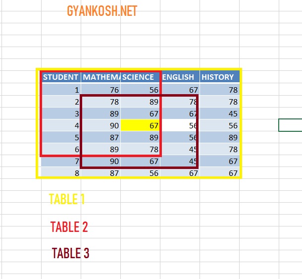
A cell is filled with YELLOW COLOR which we want to find. Now let us see in how many ways we can get this value.
The row and column number of the INDEX FUNCTION is relative to the RANGE SELECTED.