Table of Contents
- INTRODUCTION
- PURPOSE OF MATCH IN GOOGLE SHEETS
- PREREQUISITES TO LEARN MATCH
- SYNTAX FORMULA OF MATCH FUNCTION IN GOOGLE SHEETS
- EXAMPLE : MATCH FUNCTION IN GOOGLE SHEETS
- CONFUSION CLARIFICATIONS
INTRODUCTION
Looking up for values in reports is one of the most important tasks in GOOGLE SHEETS which we’d be needing to do frequently.
So the group of functions which help us for this task are the most important clan of the functions.
In this article we’ll be discussing about the FUNCTION MATCH in GOOGLE SHEETS.
MATCH FUNCTION comes under the LOOKUP group of functions in GOOGLE SHEETS.
MATCH FUNCTION looks up VALUE_TO_BE_FOUND in the given range and returns its relative position. Simply speaking, it’ll provide the relative position by matching the given values in the given table.
Relative position is the position with respect to the selected LOOKUP_RANGE.
e.g.
Suppose we have five COLORS and five CODES and we need to find out at which position ,any specified color is present.
The lookup value will be color code, and the lookup range will again be the color code complete array [all the selection from which we want to search the value from].
The result will be the relative position of the color with respect to the selection. The example will make it
more clear.
The article will describe the syntax, purpose and finally the worked out examples of the MATCH FUNCTION.
Let us start.
PURPOSE OF MATCH IN GOOGLE SHEETS
MATCH FUNCTION searches for a specified item in a range of cells and returns the relative position.
MATCH function is of utmost importance as it searches for a given value and returns its location, which we take as the input for other functions like INDEX to search for a particular value.
This kind of functions, which returns the locations are very few in GOOGLE SHEETS, which makes it very important for us to learn this function.
This function can be used anywhere , where we need to find out the position of a particular given value.
PREREQUISITES TO LEARN MATCH
THERE ARE A FEW PREREQUISITES WHICH WILL ENABLE YOU TO UNDERSTAND THIS FUNCTION IN A BETTER WAY.
- Basic understanding of how to use a formula or function.
- Easier to understand if user already knows how to use VLOOKUP.
- Basic understanding of rows and columns in GOOGLE SHEETS.
- Of course, GOOGLE SHEETS availability and internet .
Helpful links for the prerequisites mentioned above
What Excel does? How to use formula in Excel?
SYNTAX FORMULA OF MATCH FUNCTION IN GOOGLE SHEETS
The syntax ( the way how formula is phrased for excel) of MATCH FUNCTION in Excel is
=MATCH (VALUE TO BE FOUND , LOOKUP RANGE/ARRAY , MATCH MODE )
VALUE TO BE FOUND The value to be matched and found.
LOOKUP RANGE/ARRAY The range of cells, where we will try to find the match.
An array to be specific. Only one column should be selected. Else, the error would appear.
MATCH MODE
0 – Exact match. If none found, return #N/A.
-1 – Exact match. If none found, return the smallest value greater than or equal to VALUE TO BE FOUND. [The lookup range/array should necessarily be in descending order otherwise wrong answer or #N/A error can appear.
1 – Exact match.[DEFAULT] If none found, return the largest value less than or equal to the VALUE TO BE FOUND.[The lookup range/array should necessarily be in Ascending order otherwise wrong answer or #N/A error can appear.
*MATCH MODE is optional. The default value will be taken as 1 if mode is not mentioned.
EXAMPLE : MATCH FUNCTION IN GOOGLE SHEETS
DATA SAMPLE
We have two columns having the codes and colors.
We’ll use the MATCH FUNCTION in different ways to find out the relative position of the value to be found.
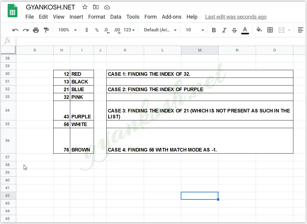
The data is put in GOOGLE SHEETS in the following fashion.
| CODES | COLORS |
|---|---|
| 12 13 21 32 43 56 76 | RED BLACK BLUE PINK PURPLE WHITE BROWN |
FOUR CASES HAVE BEEN DISCUSSED.
CASE 1: FINDING THE INDEX OF 32.
CASE 2: FINDING THE INDEX OF PURPLE
CASE 3: FINDING THE INDEX OF 21 (WHICH IS NOT PRESENT AS SUCH IN THE LIST)
CASE 4: FINDING ANY RANDOM DATA WITH MATCH MODE AS -1.
STEPS TO USE MATCH FUNCTION
STEPS TO USE MATCH FUNCTION IN GOOGLE SHEETS.
- Select the cell where you want the result.
- Use the function =MATCH(value to be matched, array in which the index is to be found, match type )
- The result will appear.
Individual examples are discussed with explanation.
CASE 1 : EXPLANATION
THE DISCUSSION IS ABOUT THE EXAMPLE SHOWN AND DISCUSSED ABOVE.
The table consists of CODES AND COLORS from the cells H20 TO I36. (WE GIVE THE STARTING AND ENDING CELL OF A TABLE WHENEVER ANY TABLE ADDRESS IS GIVEN).
CASE 1: FINDING THE INDEX OF 32.
As we can see 32 is on the number 4 in the CODES list.
The function used is
=MATCH(32,H30:H36,0)
32 is the value to be searched for . H30 :H36 is the lookup range, and 0 is the match m ode i.e. exact match.
The result comes out to be 4 which is evident as 32 is at number 4.
CASE 2: EXPLANATION
THE DISCUSSION IS ABOUT THE EXAMPLE SHOWN AND DISCUSSED ABOVE.
The table consists of CODES AND COLORS from the cells H20 TO I36. (WE GIVE THE STARTING AND ENDING CELL OF A TABLE WHENEVER ANY TABLE ADDRESS IS GIVEN).
CASE 2: FINDING THE INDEX OF PURPLE.
As we can see PURPLE is on the number 5 in the COLORS list.
The function used is
=MATCH(“PURPLE”,I30:I36,0)
PURPLE is the value to be found, next is the range and 0 is the mode. “” is used as PURPLE is a text.The result comes out to be 5.
CASE 3 & 4 : EXPLANATION
THE DISCUSSION IS ABOUT THE EXAMPLE SHOWN AND DISCUSSED ABOVE.
The table consists of CODES AND COLORS from the cells H20 TO I36. (WE GIVE THE STARTING AND ENDING CELL OF A TABLE WHENEVER ANY TABLE ADDRESS IS GIVEN).
CASE 3: FINDING THE INDEX OF 31.
31 is not in the list but this function gives us the option of finding nearest value to the value to be found.
The function used is=MATCH(31,H30:H36,1)
The value to be found is 31.
The search range is H30:H36.
Match mode is 1 which will search the value which is not higher than 31.
The codes are already in ASCENDING ORDER ( which is a must for this mode 1 and descending for -1) the result is 3 which is the nearest value smaller than the lookup_value.
CASE 4: FINDING ANY RANDOM DATA WITH MATCH MODE AS -1.
We try to find 55 using the match mode -1 which will return #N/A error as the lookup range is not in descending order.
DO YOU KNOW
EXCEL FORMULAS WORKS RELATIVELY. IF WE DRAG ANY FORMULA, IT’LL CHANGE THE CELL ADDRESSES RELATIVELY
CONFUSION CLARIFICATIONS
MATCH_MODE IN MATCH FUNCTION
The mode is chosen as 0,1 or -1
0 is simply the exact match. If the value is not found #N/A will be returned showing that the value is not available.
1 mode finds out the nearest match, if exact not found, but lesser than the lookup value whereas
-1 mode also finds out the nearest match , if exact not found, but higher than the lookup value.
The values need to be essentially in ascending order while using mode 1 and in descending order while using mode -1 otherwise wrong results will appear.
*We found many resources over net which have some problem in these modes. Kindly be careful.