Whenever we prepare any report in GOOGLE SHEETS , generally we have two constituents in any report.
The Text portion and the Numerical portion.
But just storing the text and numbers doesn’t make the super reports. Many times we need to automate the process in the reports to minimize the effort and improve the accuracy.
Many functions are provided by the GOOGLE SHEETS which work on Text and give us the useful output as well. But few problems are still left on which we need to apply some tricks with the available tools.
In this articles , we are going to separate or split the cells’ content into different parts in google sheets .
WHAT IS MEANT BY SPLITTING THE CELL
In Google Sheets, we perform a lot of activities. Out of which, cleaning the data is one of the most important activities.
For Example, we took the output as a spreadsheet file and we need to perform any operations on it, the file is not always ready to be used. It may contain the white spaces, some hidden characters or any other character which is not visible and can create problems for our functions.
ONE OF THE OPERATIONS WHICH MIGHT BE NEEDED IS SPLITTING THE CELL WHICH MEANS TO SPLIT THE CONTENT OF THE CELL ON THE BASIS OF SOME SEPARATOR. FOR EXAMPLE A SPACE, A COMMA, COLON OR ANY OTHER CHARACTER.
Suppose we took the output as a spreadsheet file and any column is containing the first name and last name of the persons in the same cell. We want to separate them.
For example, Johan Abraham,
George Butler.
Both the names are in the same column. If we want them to be in the separate columns, we need to SPLIT THE CELLS.
DIFFERENT WAYS TO SPLIT CELL IN GOOGLE SHEETS
THERE ARE MANY EASY WAYS TO SPLIT THE CELLS IN GOOGLE SHEETS.
This can be stated as removing any portion of the text or string from the cell and place it into other cells.
Cell can be split in many ways. For example
- TEXT TO COLUMN– We can split the text in a cell into the different columns. The basis of the separation can be any delimiter like a comma, colon, space etc.
- USING SPLIT FUNCTION.
- Splitting the cell into many portions.
1. SPLIT CELLS IN GOOGLE SHEETS USING TEXT TO COLUMN OPTION
We’ll discuss it here briefly as a complete detailed topic is already present.
CLICK HERE TO CHECK OUT THE COMPLETE ARTICLE ON TEXT TO COLUMN.
Text to column is used in a situation when we need to split any string [sentence or few words] separated by any delimiter [ comma, colon , full stop, semicolon, space etc. ]
The process is backed up by a wizard mechanism which makes it very simple. The only requirement is that it needs a delimiter, some character on the basis of which it’ll separate the string into words. Let us take an example to learn the way we can split cells in google sheets using Text to Column.
EXAMPLE – TEXT TO COLUMN
Let us take an example and split it with the help of TEXT TO COLUMN.
A certain case of incompatibility occurs when we download a spreadsheet from another software such as SAP.
One of the problem which I have faced is regarding the Dates.
Many times, the format of the date is not recognized by the Google Sheets and we can’t do anything about it.
Most of the data is depending upon the dates and if we can’t even sort the date, we are helpless.
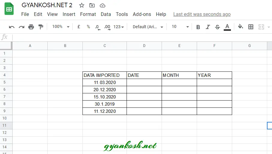
Suppose we get the dates which are in the following format.
11.03.2020
20.12.2020
15.10.2020
30.1.2019
11.12.2020
The following picture shows the data in google sheets.
STEPS TO USE TEXT TO COLUMN TO SEPARATE THE TEXT INTO COLUMNS
- As, the first column is also included in the results of TEXT TO COLUMN, we copy the text to be split into the DATE COLUMN so that the DAY coincides with the output.
- Select the complete column from D5:D9.
- Go to DATA MENU > SPLIT TEXT TO COLUMNS.

- Google Sheets will create a small popup asking for the separator.
- Click the dropdown and click on FULL STOP from the list as shown in the picture below.

- As soon as , FULL STOP is clicked, the output will appear in all the columns.
- DATE COLUMN will contain the DAY of the month, MONTH column will contain the MONTH and YEAR COLUMN contains YEAR from the given data.
The final result is shown below in the picture.

2. SPLIT CELLS IN GOOGLE SHEETS USING SPLIT FUNCTION OPTION
We’ll discuss it here briefly as a complete detailed topic is already present.
CLICK HERE TO CHECK OUT THE COMPLETE ARTICLE ON SPLIT FUNCTION
SPLIT FUNCTION IS AN IN BUILT FUNCTION IN GOOGLE SHEETS WHICH ALLOW US TO DIVIDE THE TEXT ON THE BASIS OF POSITION OF ANY DELIMITER OR SEPARATOR [ comma, colon , full stop, semicolon etc. ]
We can make use of this function in a very convenient way.This function will help us perform the same task which is done by TEXT TO COLUMN.Let us take an example to learn the use of SPLIT FUNCTION to split the cell in google sheets.
EXAMPLE- SPLIT CELL USING SPLIT FUNCTION
Let us take an example and split it with the help of SPLIT FUNCTION.
We are taking the same example as in the previous section where we used TEXT TO COLUMN option.
A certain case occurs when we download a spreadsheet from another software such as SAP.
One of the problem which I have faced is regarding the Dates.
Many times, the format of the date is not recognized by the Google Sheets and we can’t do anything about it. Most of the data is depending upon the dates and if we can’t even sort the date, we are helpless.
Suppose we get the dates which are in the following format.
11.03.2020
20.12.2020
15.10.2020
30.1.2019
11.12.2020
STEPS TO SPLIT THE CELLS INTO COLUMNS IN GOOGLE SHEETS USING SPLIT FUNCTION
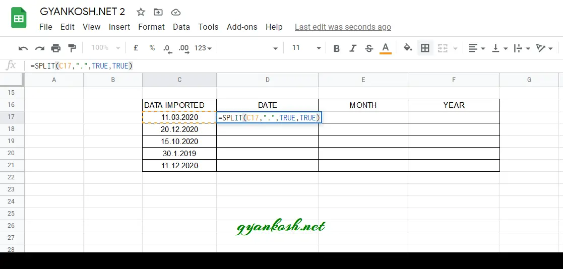
- Select the cell where we want the result. [ It’ll be the first column where first fragment will appear. Rest will appear in the adjacent columns ]
- Enter the formula as =SPLIT(C17,”.”,TRUE,TRUE).
- Click ENTER.
- All the three columns DATE , MONTH and YEAR will be filled by Day, Month and Year respectively.

- Now, drag down formula from D column through D21.
- All the data will appear correctly.

EXPLANATION
Let us understand the function usage.
For the first row, we used the formula as =SPLIT(C17,”.”,TRUE,TRUE)
The first argument is the cell containing the Text.
The second argument is the separator which is separating our text. It is a full stop passed inside the double quote.
The third argument is TRUE which will separate the text into fragment at the positions of the separator.
The fourth and last argument is TRUE which will remove any empty cell from the results.
3. SPLIT CELLS INTO CUSTOM SIZE IN GOOGLE SHEETS
Till now, we learnt two ways of splitting the cells in google sheets.
One is TEXT TO COLUMN OPTION, second one is the use of SPLIT FUNCTION.
The limitation of both the option is that they need a delimiter for their operation.
What if we have a situation where we don’t have any delimiter.
We’ll make use of the three Extremely useful functions LEFT, RIGHT and MID .
LEFT FUNCTION has the capability to pick the specified number of characters from the left side of the text.
RIGHT FUNCTION can extract the specified number of characters from the right whereas
MID FUNCTION takes out the specified number of the characters from the middle of the text.
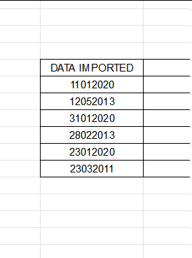
Suppose, we get these dates without any delimiter as
11012020
12052013
31012020
28022013
23012020
23032011
Let us try to find out the way to split cells in different cells.
STEPS TO SPLIT THE CELLS INTO CUSTOM SIZE
- Select the cell D28 i.e. the cell where we want to enter the DAY.
- Enter the function as =LEFT(C28,2)
- Select the cell E28.
- The day will appear.
- Enter the function as =MID(C28,3,2)
- The Month will appear.
- Select the cell F28 .
- Enter the function as =RIGHT(C28,4).
- The Year will appear.
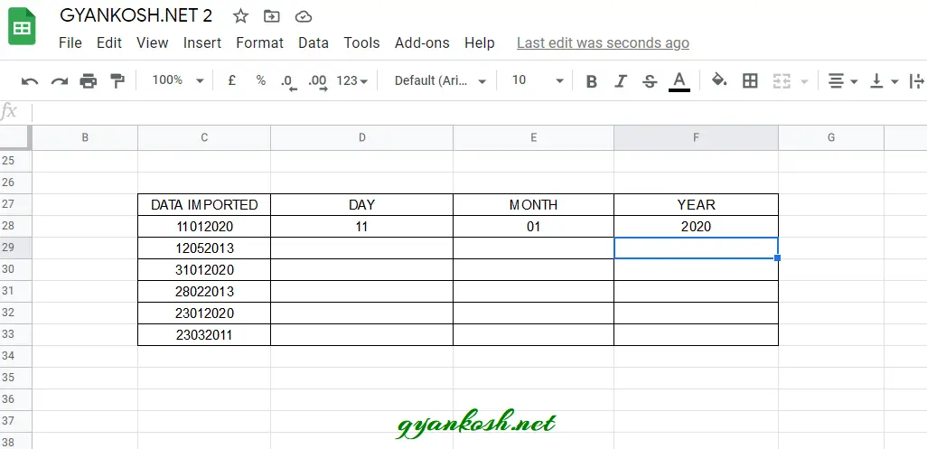
- Drag down the formula from the cell D28 through D33.
- All the cells will be filled with the formula results.
- We have successfully separated all the imported dates into day, month and year.
- Now, we can sort the date, month or year separately or we can use the DATE function to assemble the date again properly.
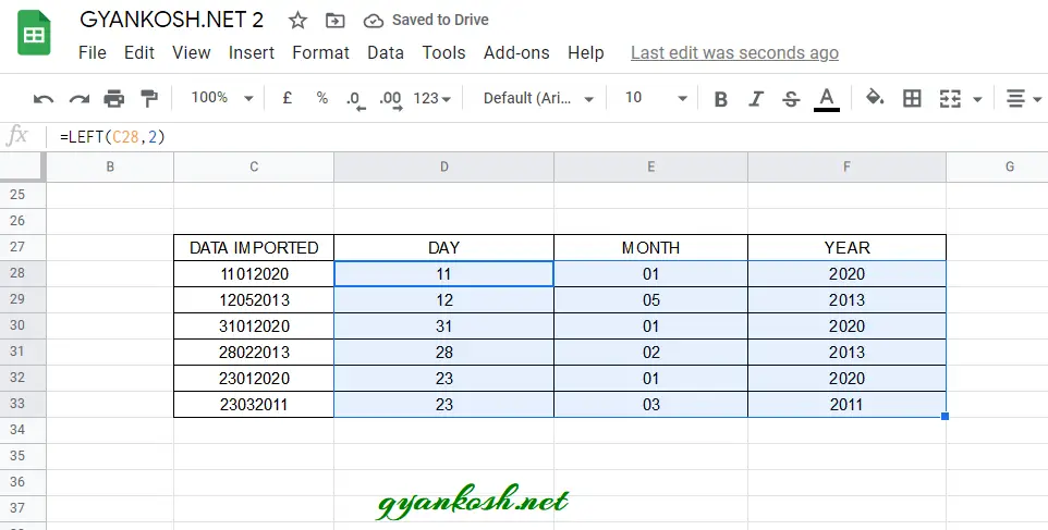
EXPLANATION
The function used for the DAY COLUMN is =LEFT(C28,2)
The first argument is the cell containing the imported date.
The second argument is the number of characters from the left side which will be kept and everything else will be removed.
The function used for the MONTH COLUMN is =MID(C28,3,2)
The first argument is the cell containing the imported date.
The second argument is the number of characters from the left side which will be kept and everything else will be removed.
The function used for the YEAR COLUMN is =RIGHT(C28,4)
The first argument is the cell containing the imported date.
The second argument is the number of characters from the left side which will be kept and everything else will be removed.