Table of Contents
- INTRODUCTION
- WHAT IS A CALCULATED FIELD IN GOOGLE SHEETS
- HOW TO INSERT A NEW CALCULATED FIELD IN GOOGLE SHEETS
- STEPS TO INSERT A NEW CALCULATED FIELD IN GOOGLE SHEETS
INTRODUCTION
PIVOT TABLE is a well known feature of EXCEL which everybody of us might have heard of. But many times we don’t know how to effectively use the PIVOT TABLE.
PIVOT TABLE is a dynamic table which we can create in Excel. We called it dynamic as we can transform it within seconds. The original data remains the same.
We know that whatever is hinged to a pivot, can rotate here and there, so is the name given to these tables.
PIVOT Table is a very powerful tool to summarize, analyze explore the data in very simple steps. Its very important to learn the use of pivot tables in excel if we want to master excel. Pivot tables give us the facility to put different simple operations on a selected data in seconds.
We have already learnt about creating PIVOT TABLES HERE.
In this article we would focus upon the situation when we need a new column in the PIVOT TABLE. The data of the column will be based upon a calculation from the already present columns.
WHAT IS A CALCULATED FIELD IN GOOGLE SHEETS
When we create a PIVOT TABLE from the given data, we have the choice of putting the information into different rows or columns.
What if we want to manipulated the data and create some new information in the PIVOT TABLE itself.
For this problem, we have got the option of inserting the CALCULATED FIELD.
A CALCULATED FIELD IS A COLUMN WHICH CAN BE INSERTED IN A PIVOT TABLE AND ANY CUSTOM CALCULATION CAN BE DONE IN THAT CUSTOM CALCULATION.
HOW TO INSERT A NEW CALCULATED FIELD IN GOOGLE SHEETS
We already learnt how to create a PIVOT TABLE . [ CLICK HERE ]
LET US TAKE AN EXAMPLE TO LEARN THE PROCESS OF INSERTING THE CALCULATED FIELD IN PIVOT TABLE.
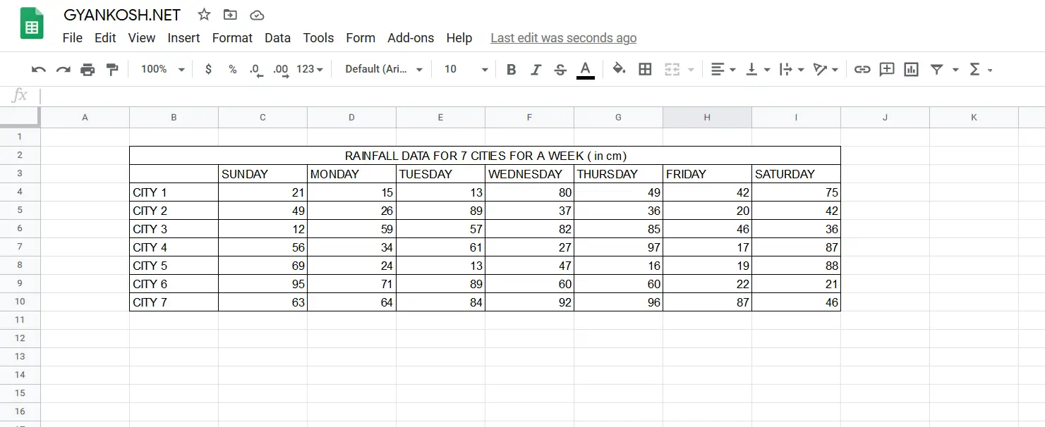
Let us find out the Maximum and Minimum Rainfall of every cities in the given week.For understanding this , let us take a new PIVOT TABLE from the given data.The data is about the RAINFALL for Seven cities for a week.The data is shown in the picture below.
Convert the above table into PIVOT TABLE using the standard procedure as discussed here.
STEPS TO CREATE PIVOT TABLE FOR THE GIVE INFORMATION
- Select the table including the headers.
- Click ADD under ROWS and choose COLUMN B.
- It’ll put all the Cities in the first column.
- Add all the cities using the same procedure by clicking ADD under the ROWS one by one.
- Deselect the SUBTOTAL checkbox under every row.
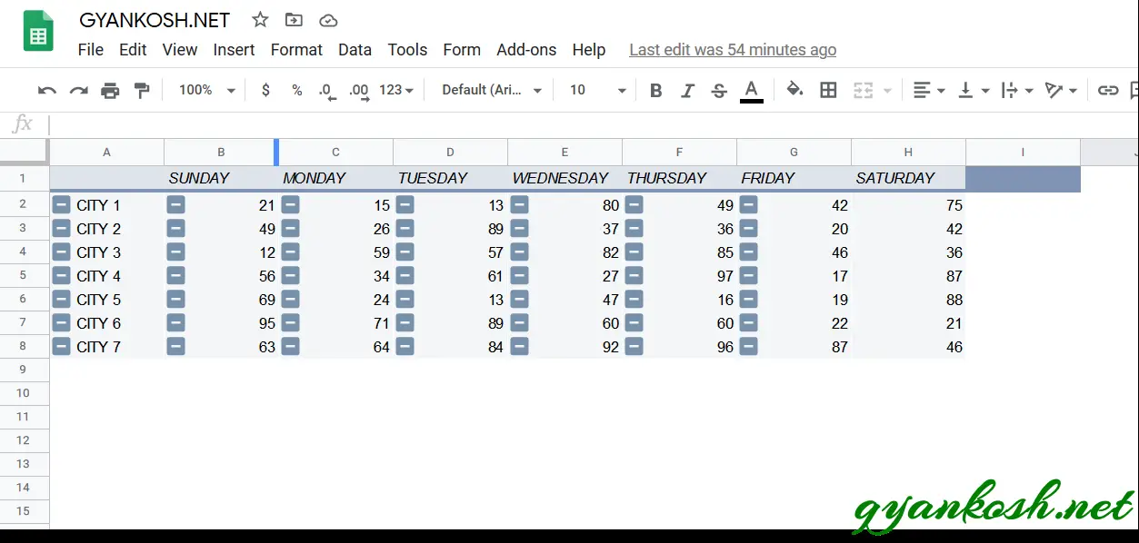
- It’ll create the pivot table in the same layout as shown in our data.
- The pivot table is shown below. [ For complete procedure click the link given in the first line. ]
STEPS TO INSERT A NEW CALCULATED FIELD IN GOOGLE SHEETS
FOLLOW THE STEPS TO INSERT A CALCULATED FIELD IN PIVOT TABLE
FINDING OUT THE MAXIMUM RAINFALL IN THE WEEK
- Click anywhere on the pivot table which will open the PIVOT TABLE EDITOR BOX on the right.
- Go to VALUES.Click ADD
- Choose CALCULATED FIELD which will be found as the last option.
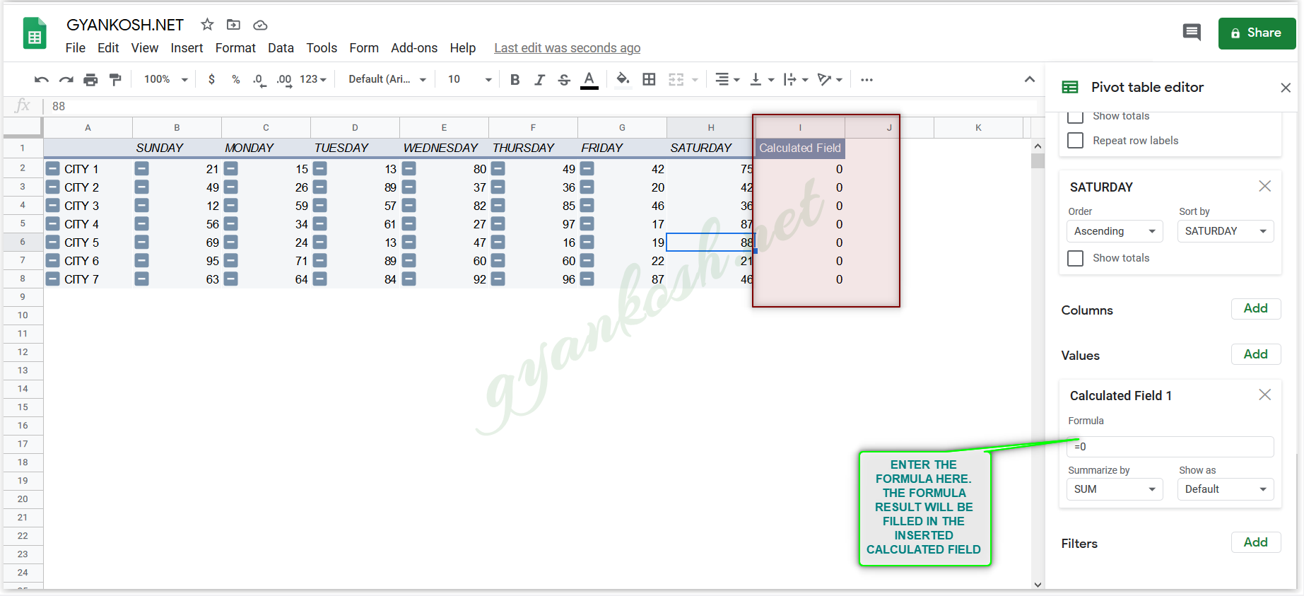
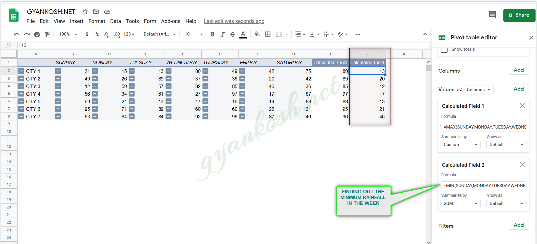
- After clicking the CALCULATED FIELD OPTION, a new column will appear in the PIVOT TABLE named as CALCULATED FIELD with 0 values.
- A field named FORMULA will open up which will need us to put the formula which will fill the values in the calculated field column.
LOOK AT THE PICTURE BELOW.
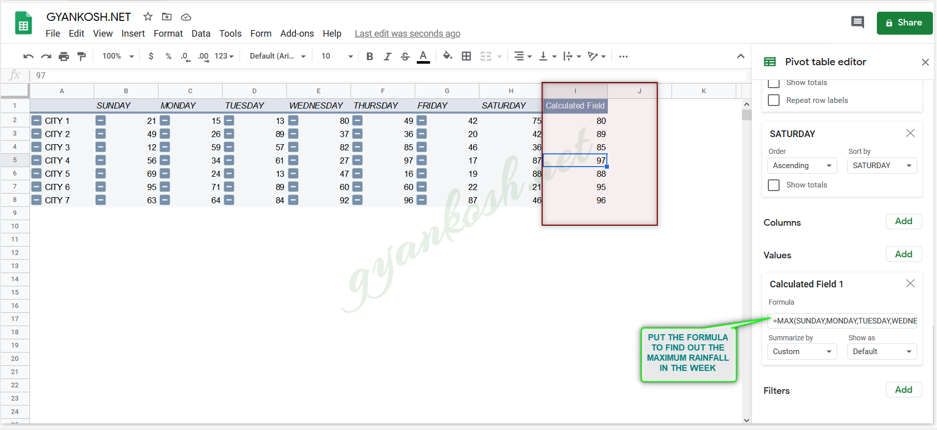
As for our example, we want to find out the maximum rainfall in the week , we’ll put the formula as
=MAX(SUNDAY,MONDAY,TUESDAY,WEDNESDAY,THURSDAY,FRIDAY,SATURDAY)
Note the formula style. We used the HEADERS to declare the formula. The individual cell addresses won’t work in the Pivot tables.
As soon as we put the correct formula, the values would fill up our column.
Let us now similarly find out the MINIMUM RAINFALL.
For the minimum rainfall, repeat the process of ADDING A CALCULATED FIELD UNDER THE VALUES and put the formula as
=MIN(SUNDAY,MONDAY,TUESDAY,WEDNESDAY,THURSDAY,FRIDAY,SATURDAY)
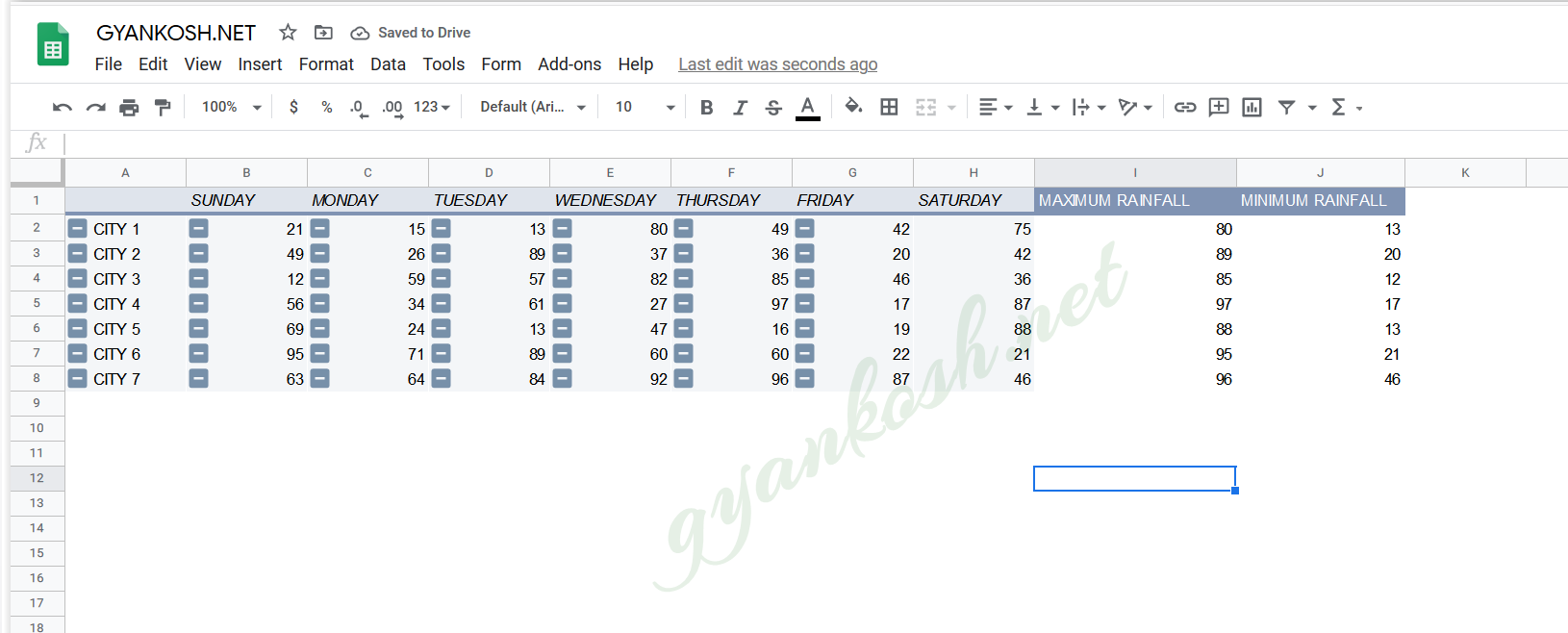
After we have created both the calculated fields, change the column names to MAXIMUM RAINFALL and MINIMUM RAINFALL.
CLICK TO LEARN HOW TO RENAME THE COLUMN IN GOOGLE SHEETS.
The final pivot table is shown below.
CALCULATED FIELDS ARE THE PART OF PIVOT TABLE NOW WITHOUT AFFECTING THE SOURCE TABLE.
