Table of Contents
INTRODUCTION
PIVOT TABLE is a well known feature of GOOGLE SHEETS which everybody of us might have heard of. But many times we don’t know how to effectively use the PIVOT TABLE.
PIVOT TABLE is a dynamic table which we can create in GOOGLE SHEETS . We called it dynamic as we can transform it within seconds. The original data remains the same.
We know that whatever is hinged to a pivot, can rotate here and there, so is the name given to these tables.
PIVOT Table is a very powerful tool to summarize, analyze explore the data in very simple steps. Its very important to learn the use of pivot tables in excel if we want to master excel. Pivot tables give us the facility to put different simple operations on a selected data in seconds.
We have already learnt about creating PIVOT TABLES HERE.
In this article we will focus upon the frequent difficulties which users face while using the pivot tables.
PROBLEM: HOW TO CHANGE COLUMN NAME OF PIVOT TABLE IN GOOGLE SHEETS
We already learnt how to create a PIVOT TABLE . [ CLICK HERE ]
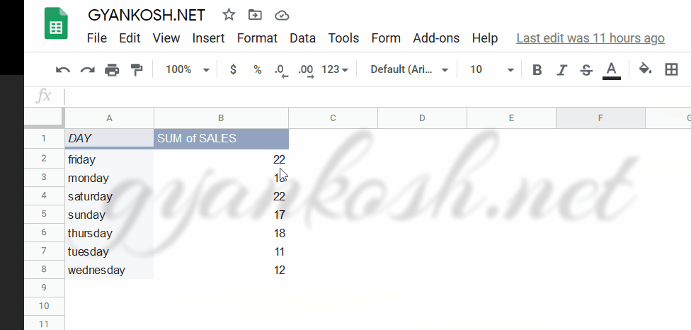
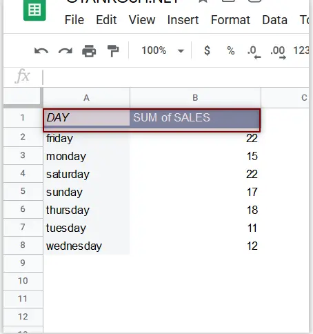
Most of the times the GOOGLE SHEETS gives the column name such as SUM OF SALES, average of sales etc.
We’ll see how we can change the column name to the desired one.
WE ASSUME THAT WE HAVE ALREADY CREATED A PIVOT TABLE.
SOLUTION:
We can see in the picture above that the PIVOT TABLE contains the column name “sum of SALES ” which is given by default by GOOGLE SHEETS.
Follow the steps to rename the column
- DOUBLE CLICK the column name in the pivot table.
- The COLUMN HEADER/NAME will become editable.
- Type the name of your choice. For our example we would type the name as “SALES”.