Table of Contents
- INTRODUCTION
- BASICS OF TIME CALCULATION IN GOOGLE SHEETS QUERY
- WHAT ARE THE DIFFERENT OPERATIONS ON TIME USING GOOGLE SHEETS QUERY?
- HOW TO AVOID PROBLEMS IN TIME FORMAT
- EXAMPLES TO USE TIME IN GOOGLE SHEETS QUERY
- EXAMPLE DATA:
- EXAMPLE 1: SHOW THE NAMES WHERE FIRST TIME IS GREATER/LATER THAN SECOND TIME SHOWING TO USE TIME IN GOOGLE SHEETS QUERY
- EXAMPLE 2: SHOW THE NAMES WHERE FIRST TIME IS BEFORE 12 NOON SHOWING TO USE TIME IN GOOGLE SHEETS QUERY
- EXAMPLE 3: SHOW THE HOURS OF THE FIRST TIME COLUMN TO USE TIME IN GOOGLE SHEETS QUERY
INTRODUCTION
In this article, we’ll learn the way to use time in Google Sheets query function.
We already learnt something about GOOGLE SHEETS QUERY LANGUAGE or GOOGLE QUERY LANGUAGE and also learnt the way to use the GOOGLE SHEETS QUERIES in GOOGLE SHEETS.
In addition to this we learnt about the various clauses in the Query language which will help us to get the data from the Google Sheets easily e.g. SELECT, WHERE, PIVOT , ORDER BY , GROUP BY and more.
This particular article is about the WHERE CLAUSE of the GOOGLE SHEETS QUERY LANGUAGE and that too about handling the TIME ONLY.
YOU CAN VISIT HERE FOR THE ESSENTIAL PREREQUISITE LEARNING OF THE WHERE CLAUSE.
DATES and TIME are quite difficult and puzzling if we don’t have proper understanding about the ways to handle them.
Here, we’d understand how to use TIME in google sheets query, add the time, subtract the time, comparison and more.
BASICS OF TIME CALCULATION IN GOOGLE SHEETS QUERY
Let us try to understand the way time is handled by Google Sheets.
As DATE is treated as the serial number [ HOW TO HANDLE DATES USING QUERIES IN GOOGLE SHEETS ? ] , time is taken as the decimal portion of the same serial number.
We know that there are 24*60*60 seconds in a day which comes out to be 86400.
So we will divide the decimal part in 86400 portions.
So one second is equal to 1/86400 which comes out to be around 0.00001157 .
One minute is equal to 1/(24*60) which comes out to be around 0.00069444.
BOTH OF THESE CALCULATIONS CAN BE CHECKED MANUALLY TOO.
Now, as we understand that the date is divided into time. It is just like the whole number is divided into the decimal.
Let us find out how it works. It is July 1, 2020 today and its serial number is 44013.
It is 10 AM at my place. Let us try to find out the fractional part so that GOOGLE SHEETS interprets it as 10 AM. [We don’t need to do this. It is just for concept building]
The counting starts from 12 AM midnight. Already 10 hrs has passed by.
10 hrs =600 minutes.
1 min= 0.00069444
600 minutes= 0.00069444×600=0.416664
Let us type in any cell of GOOGLE SHEETS.
44013.416664 and then convert the format of the cell to date and time.
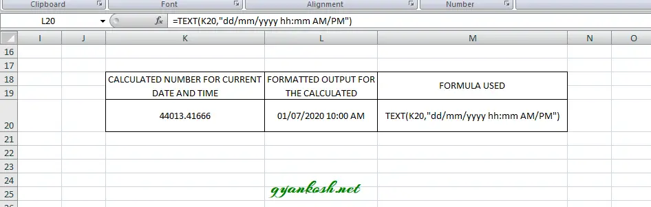
In the picture above, we can see that we put the same fractional number , which we calculated and converted it to the Date and time using the TEXT FUNCTION. The function is visible clearly. The output comes out to be the same from where we had started i.e. July 1 2020 10 AM.
REMEMBER: THE TIME CALCULATION STARTS FROM THE 12:00 AM MIDNIGHT
By this we can find out any time in the day. Some of the standard fractions are .
| TIME | FRACTION |
| 12:00 AM | 0 |
| 6:00 AM | 0.25 |
| 12:00 PM | 0.5 |
| 6:00 PM | 0.75 |
| 10:00 PM | 0.916666667 |
THE ABOVE EXCERPT HAS BEEN TAKEN FROM https://gyankosh.net/exceltricks/manipulating-date-and-time-in-excel/
WHAT ARE THE DIFFERENT OPERATIONS ON TIME USING GOOGLE SHEETS QUERY?
As we know we use the Queries to get the data shaped up as per our requirement.
We can perform a number of operations on TIME, such as
- comparing the time,
- adding the time,
- subtracting the time
and many more.
We’ll take a few examples to discuss the above-discussed points through examples.
HOW TO AVOID PROBLEMS IN TIME FORMAT
The first and foremost issue to be addressed while using the Queries based on TIME is getting the correct TIME format.
ALTHOUGH TIME FORMAT CREATES LESSER ISSUES WHEN COMPARED WITH THE DATE FORMATS BUT TAKE CARE ABOUT THE FORMATS.
If the format of the cells is not correct, the queries won’t respond properly.
CORRECT WAY OF ENTERING THE TIME IN GOOGLE SHEETS
The best way of entering the TIME in Google Sheets is the use of TIME FUNCTION. The procedure would never cause any kind of issue.
GET COMPLETE INFORMATION ABOUT TIME FUNCTION HERE.
Briefly, you can enter the time in the format by using the function.
=TIME(HOUR, MINUTES, SECONDS)
and the time will appear in the cell as per the time format selected.
Further the formats can be changed by changing the cell format easily.
FORMAT IS NOT CORRECT: For the query to work properly and return accurate data, the format of the cell should be time.
Not just format of the cell but the time entered should show a possibly correct value.
If you enter any time in a wrong format and change the format as TIME doesn’t mean that GOOGLE SHEETS will be able to process the information correctly.
So always enter the time in the proper manner in the cell , go to FORMAT BUTTON and choose as TIME.
COLUMNS WITH RANDOMLY-FORMATTED CELLS
One more issue when the queries create problems while dealing with the time is when the column containing the time is having multiple formats of data such as text, numbers , dates and more.
In this case, there can be the instances when the query function doesn’t show the error as well as won’t give the correct results.
So, in order to get the correct results, we need to take care of all the above mentioned points.
We’ll now discuss a few example to learn the proper usage of GOOGLE QUERY INVOLVING TIME.
EXAMPLES TO USE TIME IN GOOGLE SHEETS QUERY
Let us take a few examples to learn handling time in google queries.
EXAMPLE DATA:
The following table simply has the Names as A,B,C…N
A first time and a second time.
The table is somewhat like the one shown in the picture below.
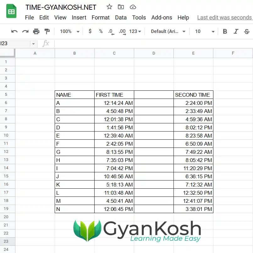
The example simply has been created for understanding time handling in Google Query.
EXAMPLE 1: SHOW THE NAMES WHERE FIRST TIME IS GREATER/LATER THAN SECOND TIME SHOWING TO USE TIME IN GOOGLE SHEETS QUERY
Let us find out the the greater or later time than the second time.
It is an example of simple comparison which might need to be found out while dealing with the times having some shifts etc., or dealing office timings etc.
In this example, we’ll simply use the comparison operator directly on the time. [ As we know that Time is simply a number ].
Simply follow the steps to find out the names which has first time is greater than second one.
- Double click the cell to make the cell editable where you want to get the result. [ In fact this will be the first cell for the result table ].
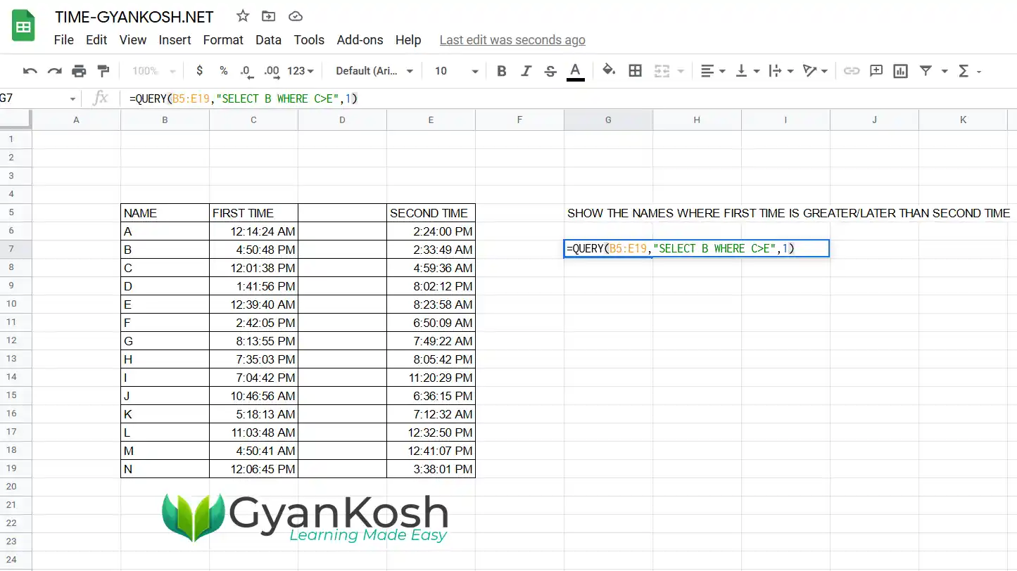
- Enter the function as =QUERY(B3:H17,”SELECT QUERY(B5:E19,”SELECT B WHERE C>E”,1).
The query used is
=QUERY(B5:E19,"SELECT B WHERE C>E",1)

The first argument is the Table containing all the data.
The Query is pretty simple. SELECT B will give B COLUMN AS OUTPUT and put the condition C>E  i.e. first time greater than second time.
Third parameter simply states to treat the top row as Header.
- After the function has been put, click ENTER to make the function execute.
The result will look like the one shown below.
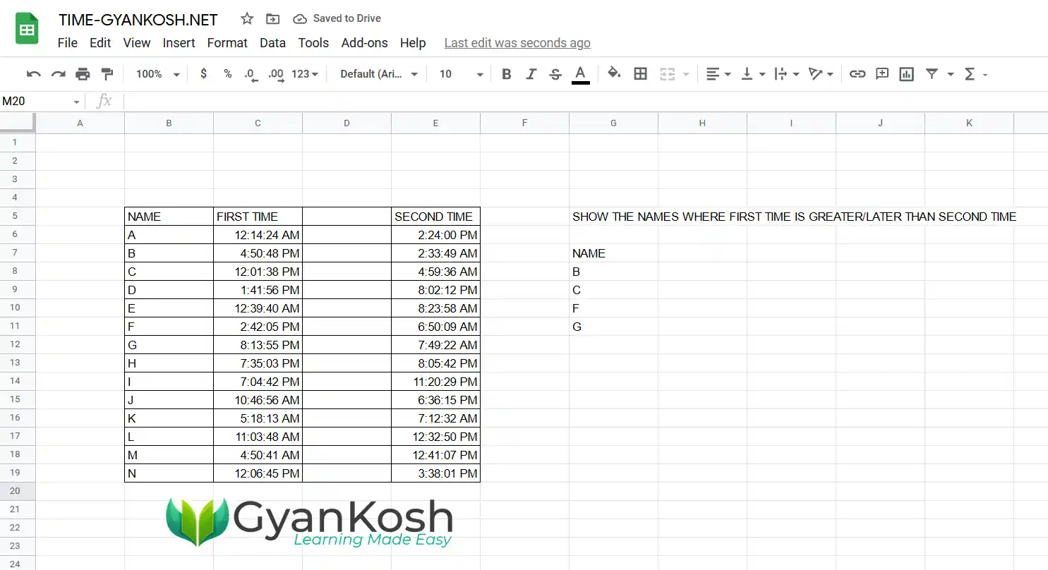
The result can be checked manually.
Let us try to find out the names which have First time lesser than 12 noon.
EXAMPLE 2: SHOW THE NAMES WHERE FIRST TIME IS BEFORE 12 NOON SHOWING TO USE TIME IN GOOGLE SHEETS QUERY
In this example, we need to find out all the time before 12 noon or 12 pm.
The major learning in this example IS TO LEARN THE WAY TO STATE THE TIME VALUE SO THAT A DIRECT COMPARISON COULD BE DONE.
WE’LL MAKE USE OF THE SORTING OF THE DATA AND TAKE OUT A SINGLE VALUE.
WE CAN COMPARE THE TIME USING THE LITERAL timeofday. [ timeofday is a literal and needs to be essentially in lower case. ]
Simply follow the steps to find out the names with first time upto 12 noon.
- Double click the cell to make the cell editable where you want to get the result. [ In fact this will be the first cell for the result table ].
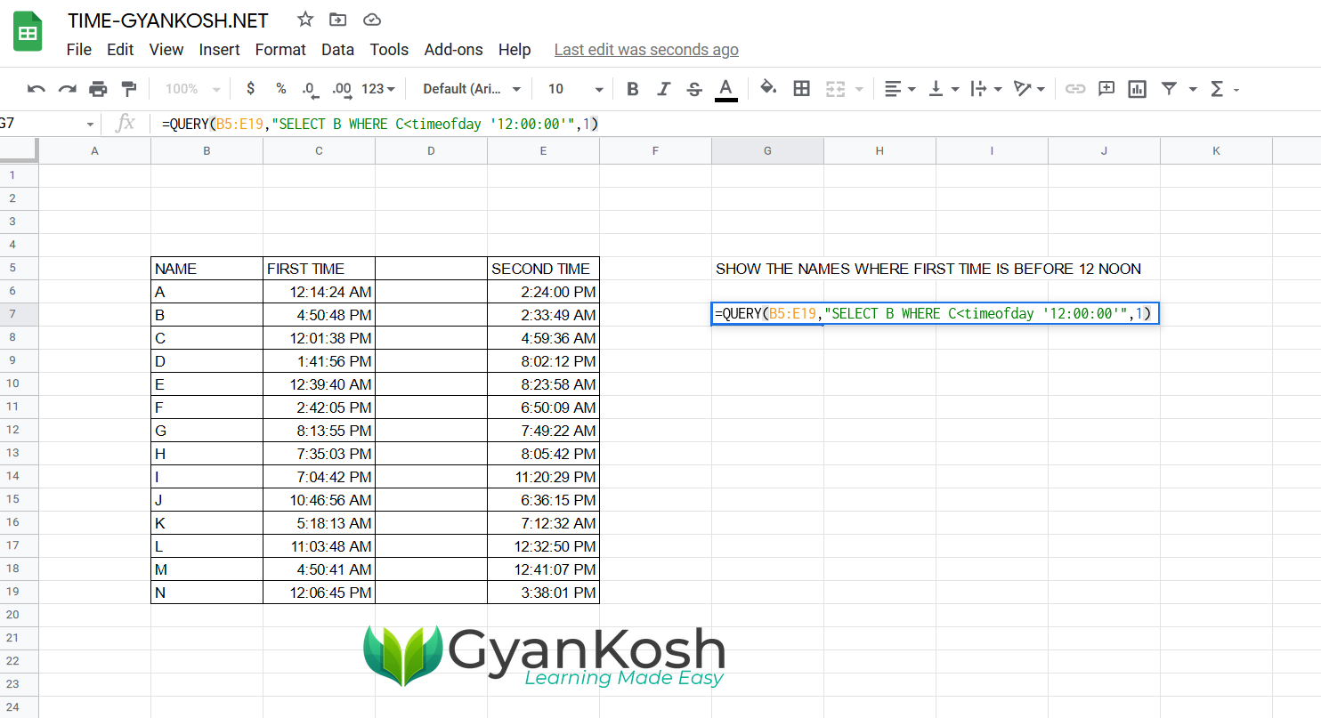
- Enter the function as =QUERY(B5:E19,”SELECT B WHERE C<timeofday ’12:00:00′”,1).
The query used is=QUERY(B5:E19,"SELECT B WHERE C<timeofday '12:00:00'",1). The first argument is the Table containing all the data. The Query is pretty simple. SELECT B will give B COLUMN AS OUTPUT and put the condition where C i.e. First time is lesser than 12:00:00. TO STATE THE TIME VALUE, literal "timeofday" is used followed with the time inside the single quotes.[ '' ] Third parameter simply states to treat the top row as Header.
- After the function has been entered, press ENTER.
- The result will appear.
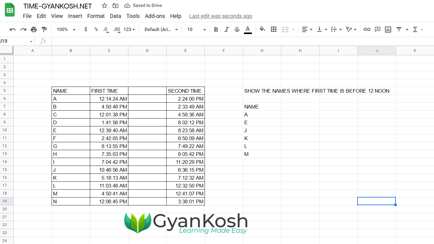
The result shows all the names where FIRST TIME is before 12 noon.
Let us take another example to learn the extraction of hour, minutes and seconds from the given data using the Queries in google sheets.
EXAMPLE 3: SHOW THE HOURS OF THE FIRST TIME COLUMN TO USE TIME IN GOOGLE SHEETS QUERY
SHOWING THE HOURS OF THE FIRST TIME:
In this example, we’ll simply extract the hours from the FIRST TIME COLUMN.
FOR GETTING THE HOURS FROM THE GIVEN TIME IN GOOGLE QUERIES, WE USE THE LITERAL hour(time) [ hour in the lower case only].
Simply follow the steps to find out hours from all the rows of FIRST TIME column.
- Double click the cell to make the cell editable where you want to get the result. [ In fact this will be the first cell for the result table ].
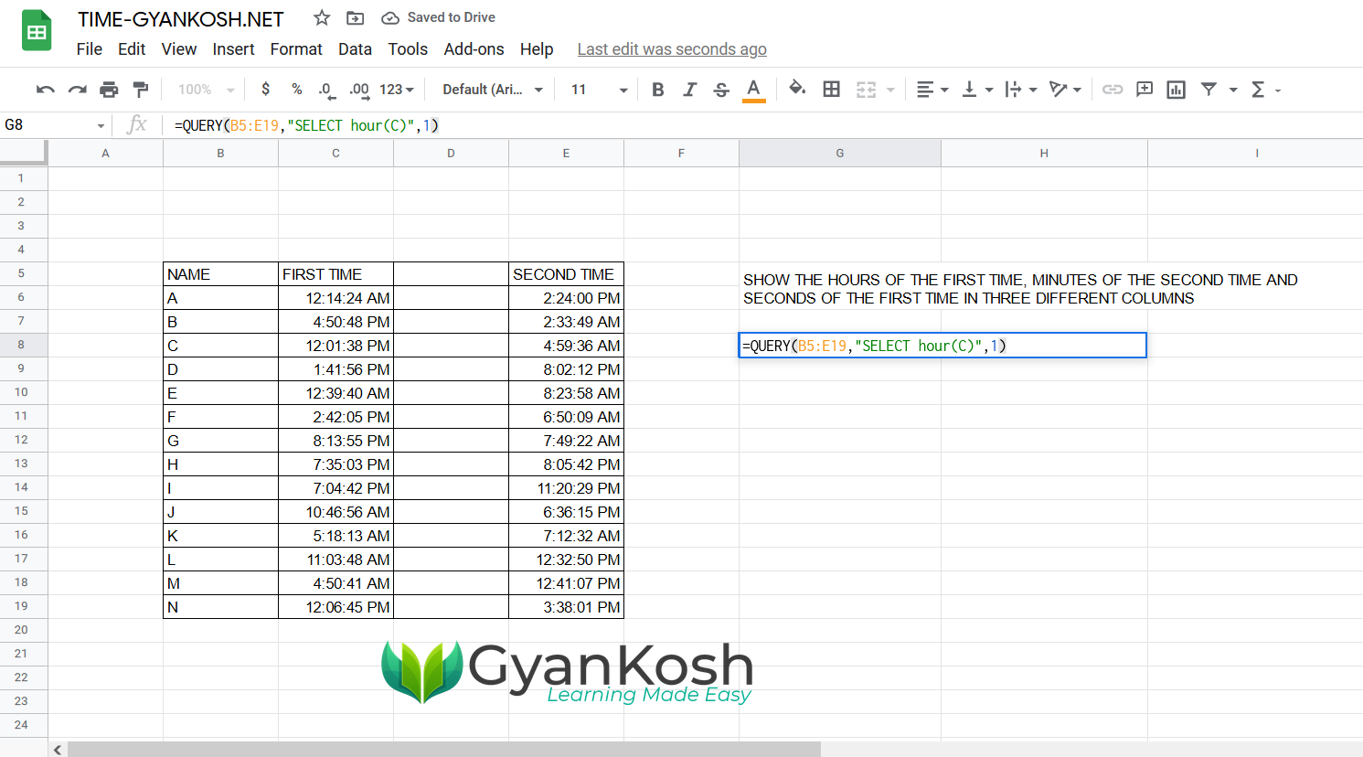
- Enter the function as =QUERY(B5:E19,”SELECT hour(C)”,1).
The query used is
=QUERY(B5:E19,"SELECT hour(C)",1)
The first argument is the data where we'll apply our query.
The Query is SELECT hour(C) which will extract the hours from the time given in column C i.e. FIRST TIME.
Last parameter shows the  number of rows as headers.
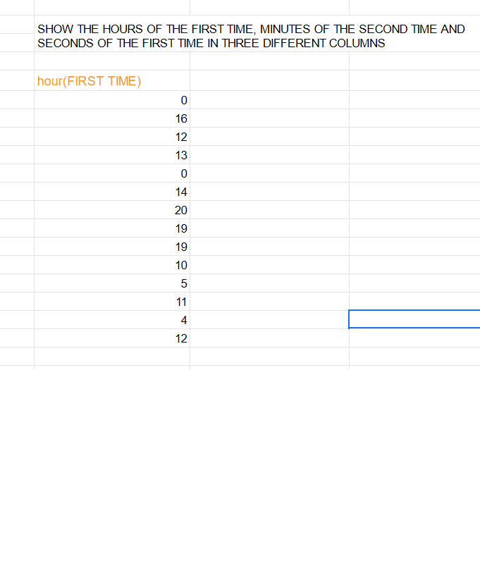
- As we enter the function, press ENTER.
- The result will appear in the form of the table as shown below.
Similarly, we’ll try to extract the minutes from the column SECOND TIME.
SHOWING THE MINUTES OF THE SECOND TIME COLUMN:
In this example, we’ll simply extract the MINUTES FROM THE SECOND TIME COLUMN.
FOR GETTING THE MINUTES FROM THE GIVEN TIME IN GOOGLE QUERIES, WE USE THE LITERAL minute(time) [ minute in the lower case only].
Simply follow the steps to find out hours from all the rows of SECOND TIME column.
- Double-click the cell to make the cell editable where you want to get the result. [ In fact, this will be the first cell for the result table ].
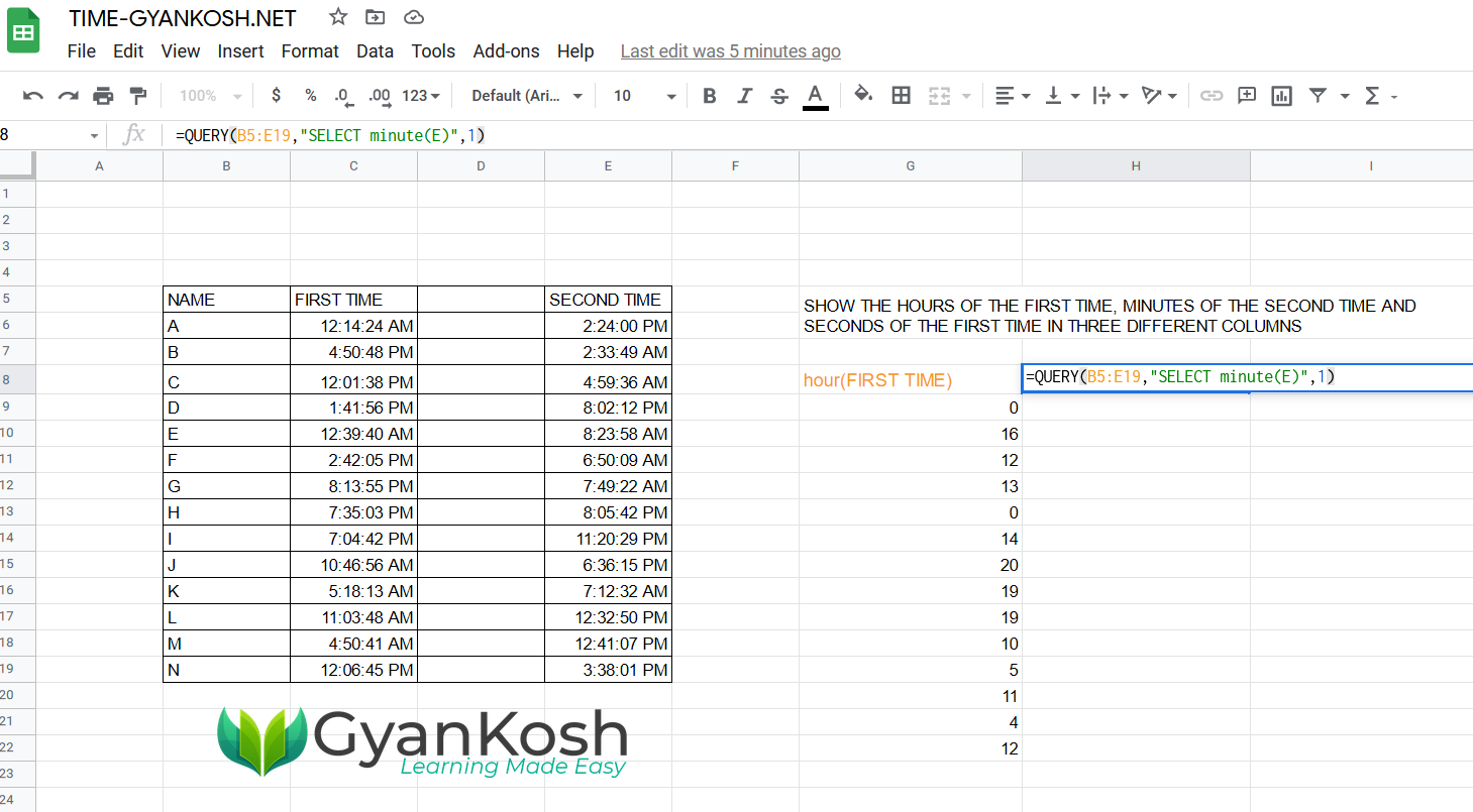
- Enter the function as =QUERY(B5:E19,”SELECT minute(E)”,1)
The query used is
=QUERY(B5:E19,"SELECT minute(E)",1)
The first argument is the data where we'll apply our query.
The Query is SELECT hour(C) which will extract the hours from the time given in column E i.e. SECOND TIME.
Last parameter shows the  number of rows as headers.
- As we enter the function, press ENTER.
- The result will appear in the form of the table as shown below.
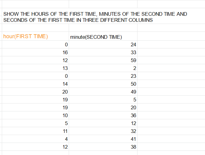
Similarly, we’ll try to extract the MINUTES from the column SECOND TIME COLUMN.
SHOWING THE SECONDS OF THE FIRST TIME COLUMN:
In this example, we’ll simply extract the SECONDS from the FIRST TIME COLUMN.
FOR GETTING THE SECONDS FROM THE GIVEN TIME IN GOOGLE QUERIES, WE USE THE Literal second(time) [ second in the lower case only].
Simply follow the steps to find out seconds from all the rows of FIRST TIME column.
- Double click the cell to make the cell editable where you want to get the result. [ In fact this will be the first cell for the result table ].
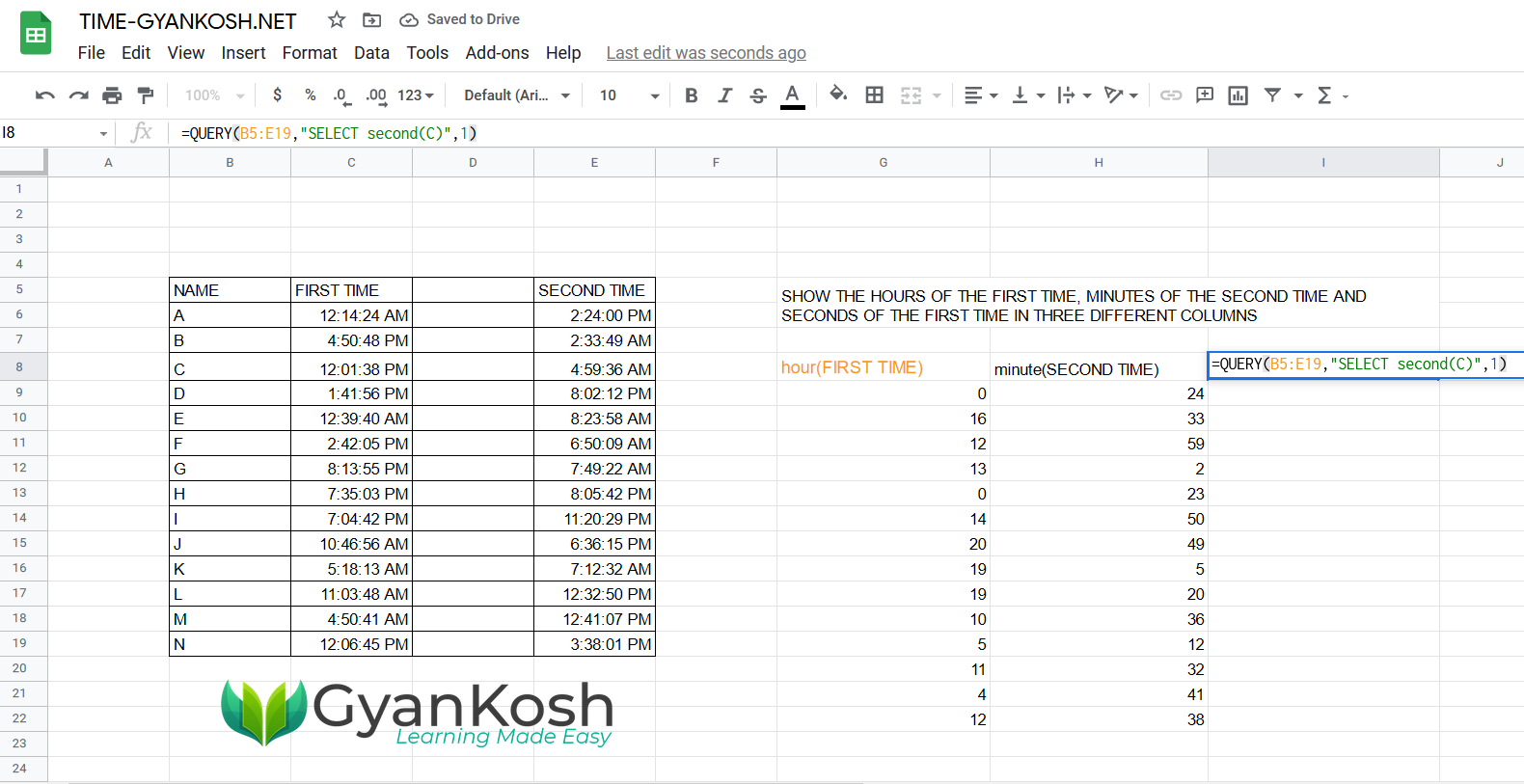
- Enter the function as =QUERY(B5:E19,”SELECT second(C)”,1).
The query used is
=QUERY(B5:E19,"SELECT second(C)",1)
The first argument is the data where we'll apply our query.
The Query is SELECT second(C) which will extract the seconds from the time given in column C i.e. FIRST TIME.
Last parameter shows the  number of rows as headers.
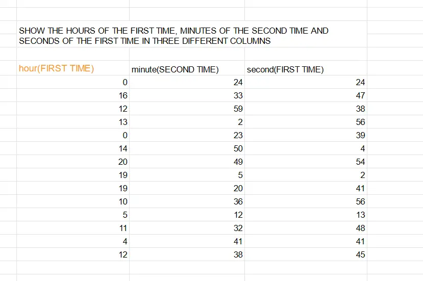
- As we enter the function, press ENTER.
- The result will appear in the form of the table as shown below.
So, in this article, we learnt the way to use time in google sheets query.