Table of Contents
- INTRODUCTION
- PURPOSE OF USING GOOGLE SHEETS QUERIES IN MULTIPLE SHEETS
- HOW TO USE THE QUERIES IN GOOGLE SHEETS FROM ONE SHEET TO ANOTHER
- EXAMPLES:
- EXAMPLE DATA:
- ISSUES:
INTRODUCTION
Google Sheets have many specific functions which are not present in other spreadsheet applications.
One of such function is a QUERY FUNCTION.
Query Function present us with the option of using the QUERIES from the GOOGLE SHEETS QUERY LANGUAGE [ Accurately GOOGLE VISUALIZATION API QUERY LANGUAGE ] to our data and save our time.
QUERY FUNCTION ENABLES US TO USE THE GOOGLE SHEETS QUERIES ON THE GIVEN DATA IN OUR GOOGLE SHEETS. THE QUERIES MAKES IT VERY SIMPLE TO EXTRACT THE COMPLETE SET OF DATA AS WE REQUIRE AND WHENEVER WE REQUIRE.
In the links shared above, you’ll learn the basics of the function and the language which is very important before you read this article.
A particular situation, when we try to QUERY from another sheet may arise during the creation of the solutions.
For this, we are writing this article.
So, in this article, we’ll learn the way to use the Query Function from a different SHEET to the other sheet.
PURPOSE OF USING GOOGLE SHEETS QUERIES IN MULTIPLE SHEETS
The purpose is very simple.
If we have data separated over the different sheets, we can easily access this data from the other sheet rather than copying the data and mixing it up with the original.
There are situations when we want to do so . For example
- If we have separate sheets for managing separate set of data.
- We don’t want to mix the data up by keeping it in the same sheet.
- Different people are using different managing sheets and you want to get particular data from the different sheets into one master sheet.
- You just want to keep the data safe by just accessing it in the viewing mode.
- To consolidate the data from different sheets
and many more.
HOW TO USE THE QUERIES IN GOOGLE SHEETS FROM ONE SHEET TO ANOTHER
For the purpose to use the Queries across the sheets in Google Sheets, we’ll be needing two important functions.
- IMPORTRANGE FUNCTION which will enable us to Import the range from the other sheet first, and
- QUERY FUNCTION which will help us to fire the query on the imported data and get the results for us.
The combination of these two functions will help us to fetch the data using the query from the other sheet.
Let us revise the functions a bit.
IMPORTRANGE FUNCTION is used to import the Range from the other sheet so that we can use it.
The syntax formula goes like =IMPORTRANGE(“URL OF THE SHEET”,”SHEET NAME! RANGE”)
This will bring the complete data table from the source to the destination.
Similarly,
Query function helps us to use the QUERY on the GIVEN RANGE.
The syntax formula goes like
=QUERY( RANGE OR DATA, QUERY, NUMBER OF HEADER ROWS)
COMBINING IMPORTRANGE AND QUERY TO GET THE QUERY OVER DIFFERENT SHEETS
We’ll put the IMPORTRANGE inside the QUERY FUNCTION to fetch the range and simply apply the QUERY to the fetched data.
So, the GENERALIZED FORMULA becomes
= QUERY ( IMPORTRANGE(” SOURCE GOOGLE SHEET URL”,” SOURCE SHEET NAME ! RANGE OF THE DATA”), ” QUERY” , NUMBER OF HEADERS)
So, using this method, we’ll be able to apply the Query in multiple sheets and perform the analysis on the brought data.
Let us try this with the help of an example.
EXAMPLES:
EXAMPLE DATA:
We have a data table in one sheet which contains the Employee data as shown in the picture below.

EXAMPLE 1: FETCH THE EMPLOYEE NAME AND ATTENDANCE FROM THE GIVEN SHEET TO THE OTHER SHEET
SOLUTION:
After we have acquired all the information we need, we can directly try the solution.
FOLLOW THE STEPS TO FETCH THE EMPLOYEE NAME AND ATTENDANCE FROM THE OTHER SHEET
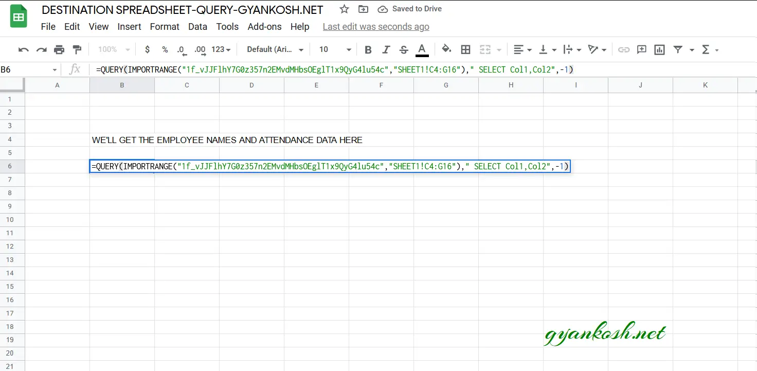
- Select the cell where you want the result.
- Enter the function as =QUERY(IMPORTRANGE(“1f_vJJFlhY7G0z357n2EMvdMHbsOEglT1x9QyG4lu54c”,”SHEET1!C4:G16″),” SELECT Col1,Col2″,-1)
The query used is
=QUERY(IMPORTRANGE("1f_vJJFlhY7G0z357n2EMvdMHbsOEglT1x9QyG4lu54c","SHEET1!C4:G16")," SELECT Col1,Col2",-1)
The first argument is in the form of IMPORTRANGE FUNCTION which will bring the complete dataset from the other sheet to the current sheet.
The second argument is simply the QUERY as if the data were present in the current sheet only.
*The only thing to be taken care of is the column names. The local column names won't work here but the columns as per the data brought through the IMPORTRANGE FUNCTION will only work. We use them as Col1 for first column, Col2 for second and so on.
The third argument is standard , the number of header rows.
- After putting the formula, press Enter.
- The data will be loaded as shown in the picture below.
ACCESS ISSUE WHILE USING IMPORTRANGE
When we use the IMPORTRANGE for the first time, the ACCESS ISSUE appears in the form of the ERROR.
Just hover over the error and choose ALLOW ACCESS.
It'll give the one sheet permission to read the other sheet.
This is important and easy at the same time.
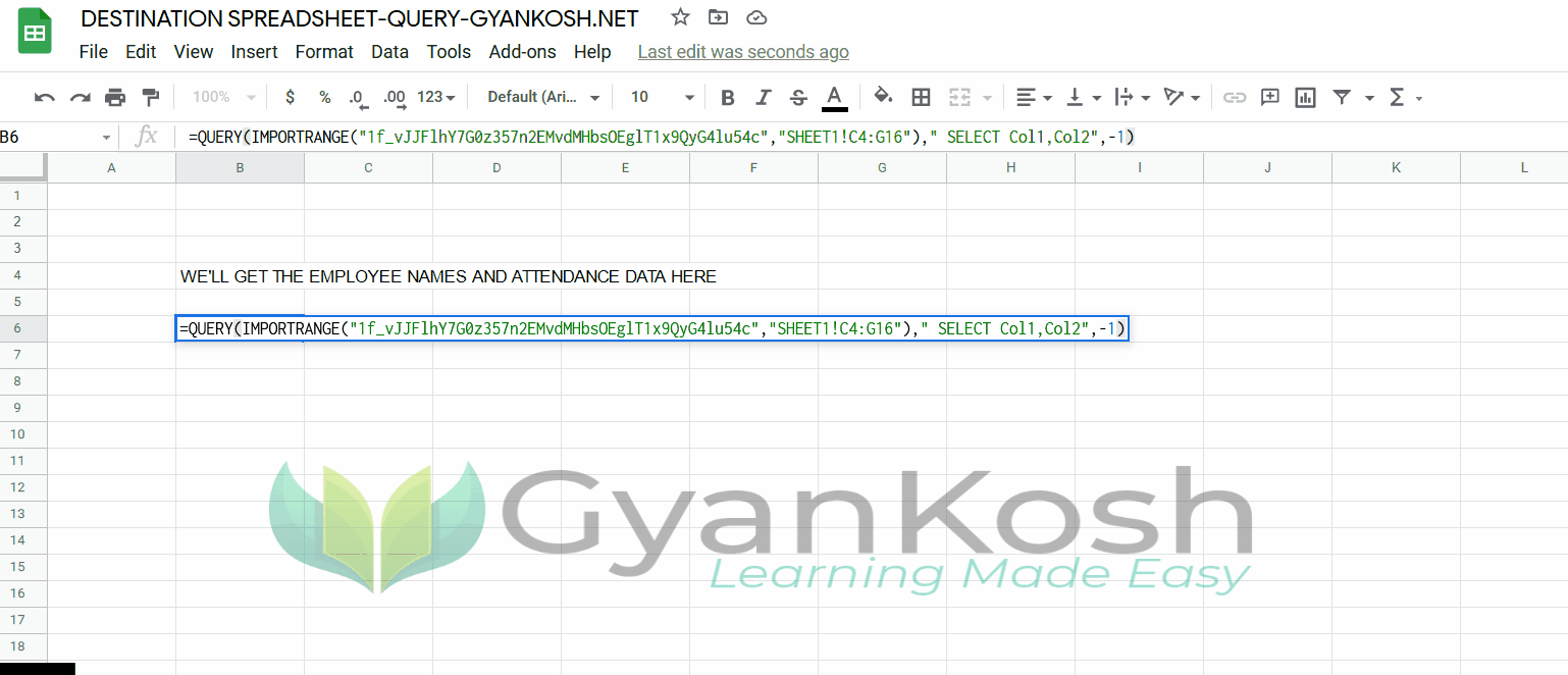
- As we click the Enter, the data is fetched simply.
This was the way to use query from the other sheet to different sheet in Google Sheets.
Let us now discuss a few points which might confuse you.
ISSUES:
1. ERROR WHILE GETTING THE RANGE.
We already discussed this earlier too, that it is simply the Security issue which is a need too.
When we are accessing the range from the other sheet, it’ll ask the user for the permission.
Get the permission and you are good to go. This will be a one time process.
2. COLUMN NAME NOT FOUND ERROR IN QUERY FOR GOOGLE SHEETS
The column names won’t work when we are getting the range through IMPORTRANGE FUNCTION.
You need to make use of the notation Col1 , Col2 and so on to address the columns.
Col1 will point towards the first column from the IMPORTRANGE FUNCTION.
Col2 will point towards the second column of the table fetched using IMPORTRANGE FUNCTION.
In this article , we learnt about the process of using the Queries through the different sheets in Google Sheets.