Table of Contents
- INTRODUCTION
- HOW DATES WORK IN GOOGLE SHEETS ?
- DIFFERENT OPERATIONS WHICH CAN BE DONE ON DATES USING GOOGLE SHEETS QUERIES
- HOW TO AVOID PROBLEMS IN DATE FORMAT
- CORRECT WAY OF ENTERING THE DATES IN GOOGLE SHEETS
- EXAMPLES
- EXAMPLE DATA:
- EXAMPLE 1: FIND OUT THE YOUNGEST EMPLOYEE- USING ORDER BY AND OFFSET
- EXAMPLE 2: FIND OUT THE OLDEST EMPLOYEE-USING ORDER BY AND LIMIT
- EXAMPLE 3: FIND OUT THE EMPLOYEES WHO JOINED BEFORE YEAR 2000- COMPARING THE DATES
INTRODUCTION
We already learnt something about GOOGLE SHEETS QUERY LANGUAGE or GOOGLE QUERY LANGUAGE and also learnt the way to use the GOOGLE SHEETS QUERIES in GOOGLE SHEETS.
In addition to this we learnt about the various clauses in the Query language which will help us to get the data from the Google Sheets easily e.g. SELECT, WHERE, PIVOT , ORDER BY , GROUP BY and more.
This particular article is about the WHERE CLAUSE of the GOOGLE SHEETS QUERY LANGUAGE and that too about handling the DATES ONLY.
YOU CAN VISIT HERE FOR THE ESSENTIAL PREREQUISITE LEARNING OF THE WHERE CLAUSE.
DATES , if you don’t understand them, can create a havoc while handling them in Google Sheets or even EXCEL.
So, in this article, we’d just focus on handling DATES.
Here, we’d understand how to work with the dates, finding out the difference of days, getting the data based upon the dates using the GOOGLE QUERIES.
HOW DATES WORK IN GOOGLE SHEETS ?
So , before proceeding further, let us find out the way dates work in Google Sheets.
The first and foremost point is to understand how Google Sheets handles the dates.
Date is treated as a simple serial number by Google Sheets starting from DEC 31 1899 [ treated as 1]. From Dec 31, 1899 which is 1 for Google Sheets the serial number starts and it is still going on . For example, it is 25th Aug 2021 today so the serial number for this date is 44433.
If we type this number in Google Sheets and convert the format to date, It’ll translate it to the date mentioned above which is 25-8-2021.
We can write the date in the various DATE FORMATS or we can simply use the numbers.[ Of course it is not easy to remember the numbers, but we can refer for once].
GOOGLE SHEETS HAS THE PROVISION OF DATES FROM DEC 31,1899 TO DEC 31, 9999 which corresponds to 2958465.
So it should be clear to the Google Sheets user that date is nothing but a number.
But why so many problems appear while using the DATES in Google Sheets?
The problems occur when we think that the given format is Date but Google Sheets doesn’t accept it as a date. It happens when we violate the rules of entering the date.
It also occurs when the data looks like a date but there is some mistake in the format.
DIFFERENT OPERATIONS WHICH CAN BE DONE ON DATES USING GOOGLE SHEETS QUERIES
As we know we use the Queries to get the data shaped up as per our requirement.
We can perform a number of operations on the dates, such as
Getting the oldest date,
Getting the latest date,
Comparing the date with any reference date
and many more.
We’ll take a few examples to discuss the above discussed points through examples.
HOW TO AVOID PROBLEMS IN DATE FORMAT
The first and foremost issue to be addressed while using the Queries based on Dates is getting the correct date format.
If the format of the cells is not correct, the queries won’t respond properly.
CORRECT WAY OF ENTERING THE DATES IN GOOGLE SHEETS
The best way of entering the date in Google Sheets is the use of DATE FUNCTION. The procedure would never cause any kind of issue.
GET COMPLETE INFORMATION ABOUT DATE FUNCTION HERE.
Briefly, you can enter the date in the format by using the function.
=DATE(YEAR, MONTH, DAY)
and the date will appear in the cell as per the date format selected.
Further the formats can be changed by changing the cell format easily.
FORMAT IS NOT CORRECT: For the query to work properly and return accurate data, the format of the cell should be date.
Not just format of the cell but the date entered should show a possibly correct value.
If you enter any date in a wrong format and change the format as DATE doesn’t mean that GOOGLE SHEETS will be able to process the information correctly.
So always enter the date in the proper manner in the cell , go to FORMAT BUTTON and choose as DATE.
IF YOU ARE CONFUSED ABOUT THE PROPER FORMAT, MAKE USE OF DATE FUNCTION.
THE STANDARD FORMAT OF THE DATE IS ONE WHICH YOUR OPERATING SYSTEM IS SHOWING IN THE BOTTOM RIGHT CORNER OR ANY OTHER PLACE. WE ALSO CALL THIS TIME AS SYSTEM TIME.
COLUMNS WITH RANDOMLY-FORMATTED CELLS
One more issue when the queries create problems while dealing with the dates is when the column containing the dates is having multiple formats of data such as text, numbers , dates and more.
In this case, there can be the instances when the query function doesn’t show the error as well as won’t give the correct results.
So, in order to get the correct results, we need to take care of all the above mentioned points.
We’ll now discuss a few example to learn the proper usage of GOOGLE QUERY INVOLVING DATES.
EXAMPLES
Let us take a few examples to learn handling dates in google queries.
EXAMPLE DATA:
The following table contains the data about the employees including their date of birth, joining date, date of retirement and experience.
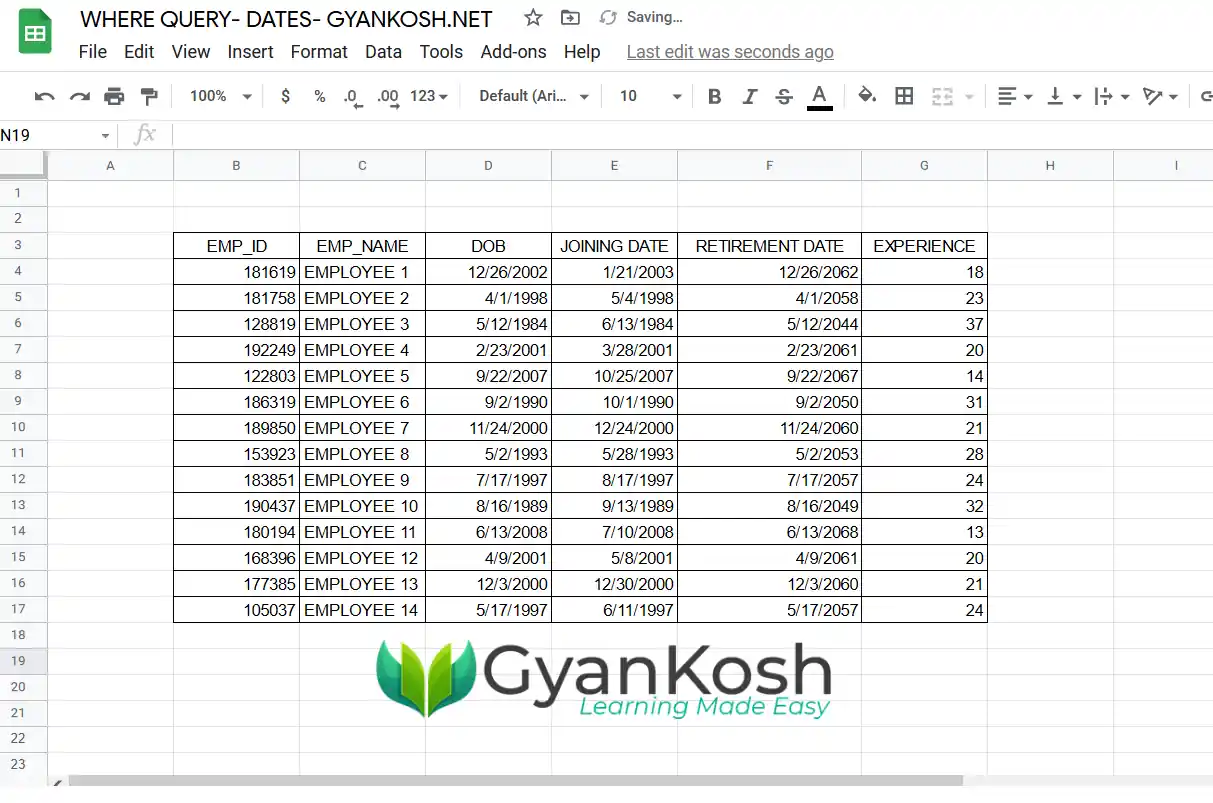
We have created many columns with the date entry so that we can use many examples to learn the system.
EXAMPLE 1: FIND OUT THE YOUNGEST EMPLOYEE- USING ORDER BY AND OFFSET
Let us find out the employee who is youngest employee.
Now, there is an issue while trying to find the youngest and oldest employee.
We can’t get a look up value from the table but we can shape up the table. So, we’ll try a trick to find out the youngest and oldest employee.
WE’LL MAKE USE OF THE SORTING OF THE DATA AND TAKE OUT A SINGLE VALUE.
THE SORTING IN THE GOOGLE SHEETS QUERY LANGUAGE CAN BE DONE WITH THE HELP OF ORDER BY CLAUSE.
Simply follow the steps to find out the employee with maximum experience.
- Double click the cell to make the cell editable where you want to get the result. [ In fact this will be the first cell for the result table ].
- Enter the function as =QUERY(B3:H17,”SELECT C,D ORDER BY D OFFSET 13″,1).
The query used is
=QUERY(B3:H17,"SELECT C,D ORDER BY D OFFSET 13",1)

The first argument is the Table containing all the data.
The query uses SELECT C,D [ enlist C COLUMN and D COLUMN ] ORDER BY D [ SORT IT BY D] OFFSET 13 [ WHERE 13 IS THE NUMBER OF ROWS-1. OFFSET WILL REMOVE THE RESULT WITH THE NUMBER OF ROWS MENTIONED ]
The description above will make it clear the trick we used.
The QUERY we used [ without offset ] will return a complete table where the date of birth of the employees are in the ascending order i.e. the oldest employee will be at the top and youngest at the bottom.

So, we removed all the rows but last row which is the required result of our problem.

- After the function has been put, click ENTER to make the function execute.
The result will look like the one shown below.
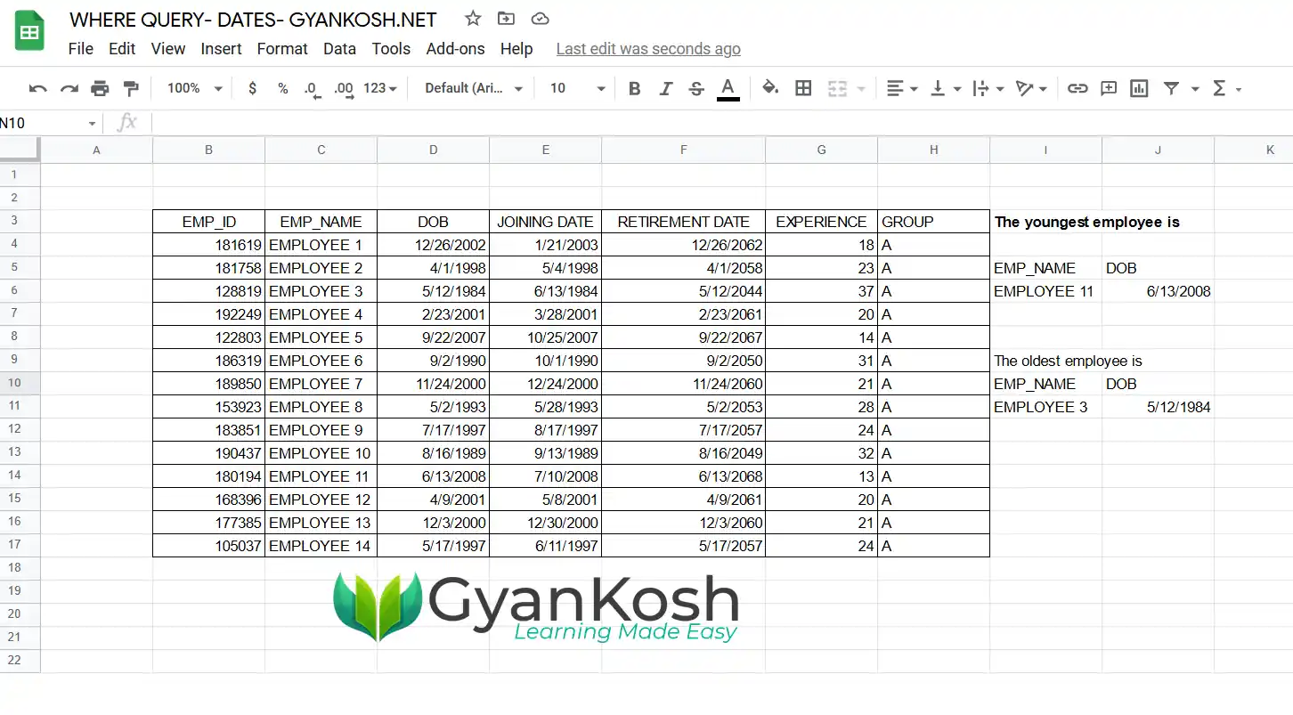
We can see that the result has shown EMPLOYEE 11 as the youngest which is correct. His date of birth is 13th June 2008.
Similarly let us try to find out the oldest employee.
EXAMPLE 2: FIND OUT THE OLDEST EMPLOYEE-USING ORDER BY AND LIMIT
Let us find out the oldest employee now.
The problem remains the same with this problem too.
We can’t get a look up value from the table but we can shape up the table. So, we’ll try a trick to find out the youngest and oldest employee.
WE’LL MAKE USE OF THE SORTING OF THE DATA AND TAKE OUT A SINGLE VALUE.
THE SORTING IN THE GOOGLE SHEETS QUERY LANGUAGE CAN BE DONE WITH THE HELP OF ORDER BY CLAUSE.
Simply follow the steps to find out the employee with maximum experience.
- Double click the cell to make the cell editable where you want to get the result. [ In fact this will be the first cell for the result table ].
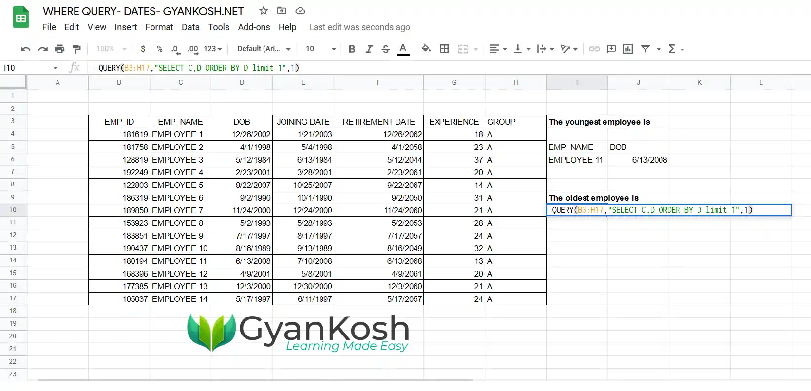
- Enter the function as =QUERY(B3:H17,”SELECT C,D ORDER BY D limit 1″,1)
The query used is
=QUERY(B3:H17,"SELECT C,D ORDER BY D limit 1",1)
The first argument is the Table containing all the data.
The query uses SELECT C,D [ enlist C COLUMN and D COLUMN ] ORDER BY D [ SORT IT BY D] LIMIT 1 [ LIMIT THE RESULT TO 1 ROW ].
The description above will make it clear the trick we used.

We demanded a complete table which was sorted on the basis of date of births, but we limited the result to one row and that row must be of the employee who was born first i.e. oldest person.
- After the function has been entered, press ENTER.
- The result will appear.
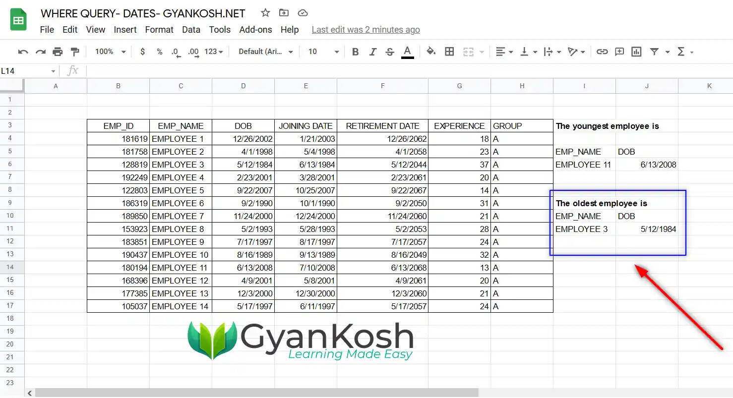
The result shows the oldest employee as EMPLOYEE 3 who was born in 1984.
Let us take another example to find out the employees who joined before a certain date.
EXAMPLE 3: FIND OUT THE EMPLOYEES WHO JOINED BEFORE YEAR 2000- COMPARING THE DATES
In this example we’ll use the simple LESS THAN operator in the query and try to find out the people who joined before 2000.
For that, follow this.
Simply follow the steps to find out the employees joined before 2000.
- Double click the cell to make the cell editable where you want to get the result. [ In fact this will be the first cell for the result table ].
- Enter the function as =QUERY(B3:H17,”SELECT C,E where E< date ‘2000-01-01′”,1)
The query used is
=QUERY(B3:H17,"SELECT C,E where E< date '2000-01-01'",1)
The first argument is the data where we'll apply our query.
The Query is SELECT C,E [ SHOW C,E IN THE REUSLT ] WHERE E [ JOINING DATE ] < [ LESSER THAN OR OLDER THAN ] date [ identifier for DATE ] '2001-01-01' [ date in the format yyyy-mm-dd].
Last parameter shows the  number of rows as headers.

- As we enter the function, press ENTER.
- The result will appear in the form of the table as shown below.
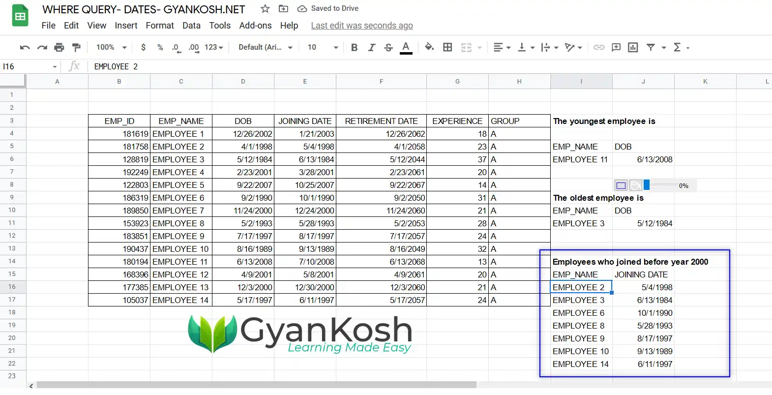
These were a few ways of using DATES in the QUERY FUNCTION in GOOGLE SHEETS to make use of GOOGLE SHEETS QUERIES.