SIMPLE WAYS TO DISABLE CELL EDITING IN GOOGLE SHEETS?

Table of Contents

• INTRODUCTION
• WHAT IS DISABLING THE CELLS, COLUMNS, OR ROWS IN GOOGLE SHEETS?
• WHY TO DISABLE CELL EDITING IN GOOGLE SHEETS?
• EXAMPLE 1: DISABLE A FEW SPECIFIC CELLS E.G. A1, B1 AND D4 IN GOOGLE SHEETS
• SOLUTION
• CHECKING THE DISABLED CELLS
• EXAMPLE 2: DISABLE EDITING IN COLUMN C IN GOOGLE SHEETS
• SOLUTION:
• CHECKING THE DISABLED COLUMN
• EXAMPLE 3: DISABLE ANY EDITING IN ROW NUMBER 6
• SOLUTION:
• CHECKING THE DISABLED ROW

INTRODUCTION

Google Sheets is a real champion when we want to share the sheets among different users. Perhaps the main reason for this ease is the need of the google account which almost every person is having now a days.

So, this article is going to discuss the ways about how to disable cell editing in Google Sheets.

DISABLING CELLS, COLUMNS OR ROWS IN GOOGLE SHEETS TO STOP THE EDITABLE PROPERTY OF THESE SO THAT SOMEBODY MIGHT NOT

CHANGE THE FORMULAS OR ANY VALUES BY MISTAKE OR INTENTIONALLY. IT IS KIND OF PROTECTING THE CELLS, COLUMNS OR ROWS FROM UNAUTHORIZED ACCESS.

FOR MORE INFORMATION ABOUT THE STANDARD PROCEDURES FOR LOCKING, UNLOCKING THE CELLS OR SHEETS , YOU CAN CLICK ANYWHERE ON THIS LINE.

In this article, we’ll learn the way to disable specific cells, columns or rows in google sheets with the help of the examples.

WHAT IS DISABLING THE CELLS, COLUMNS, OR ROWS IN GOOGLE SHEETS?

The literal meaning of DISABLING means to completely disable the cells to respond to any kind of click or any response so that no value can be stored in the cell or there is no change or editing in the cell.

But do we really need such kind of disabled cells, columns or rows.

The answer is NO!!.

Because if the cells are completely frozen, they are not of any use.

So, by disabling the cells, column,s or rows in google sheets we simply mean to

STOP THE ACCESS OF CERTAIN CELLS, COLUMNS OR ROWS FROM THE USERS SO THAT THEY MIGHT NOT EDIT OR DELETE THE CONTENT IN THE PARTICULAR CELLS.

ONLY THE USER, WHO IS CREATING THE RULE FOR PROTECTION OF CELLS, COLUMNS OR ROWS, WILL BE ABLE TO MAKE THE CHANGES. ALL OTHER USERS WILL NOT BE ABLE TO EDIT THE DISABLED CELLS BUT VIEW ITS CONTENT OR RESULTS IN THOSE CELLS, COLUMNS OR ROWS.

This is a very frequent situation when we’d like to do so.

In this article, we’d learn different techniques to do so.

WHY TO DISABLE CELL EDITING IN GOOGLE SHEETS?

Disabling the cells, columns or rows from editing might be required in many cases.

Some of them can be when-

1. We want to limit editing from the specific cells, columns or rows.
2. We want to allow only a few persons to be able to edit.
3. We want to avoid any unplanned changes.
4. We want to avoid mistakes.

and some more can be there.

The major reason is to restrict the access to the few cells , columns or rows to avoid any mistake.

A certain practical scenario can be helpful here for better understanding the need.

Suppose there is a particular format on which a number of people work.

We know very well that in any calculations there must be some raw data which is simply entered inside the cells manually.

While performing this job, there are high chances for somebody to disturb the cells with the formulas. It happens quite frequently.

If the sheets are very big, we might overlook the error generated because of this.

This is where , the locking or disabling the editing of cell, columns and rows become very beneficial to us.

Let us learn.

EXAMPLE 1: DISABLE A FEW SPECIFIC CELLS E.G. A1, B1 AND D4 IN GOOGLE SHEETS

SOLUTION

We’ll use the protection option to solve this problem and disable the cells A1,B1 and D4 so that nobody can edit the cells.

FOLLOW THE STEPS TO DISABLE THE CELLS A1,B1 AND D4.

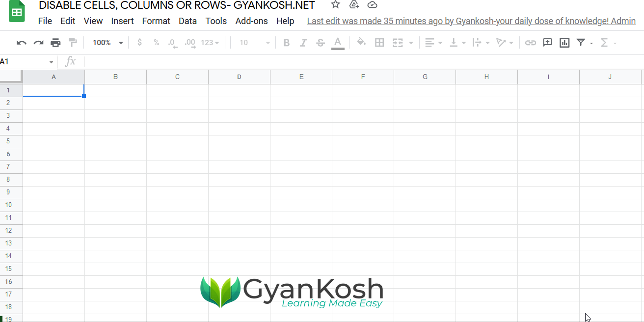
• Open the Google Sheets and create or open the sheet where you want to disable the specific cells.

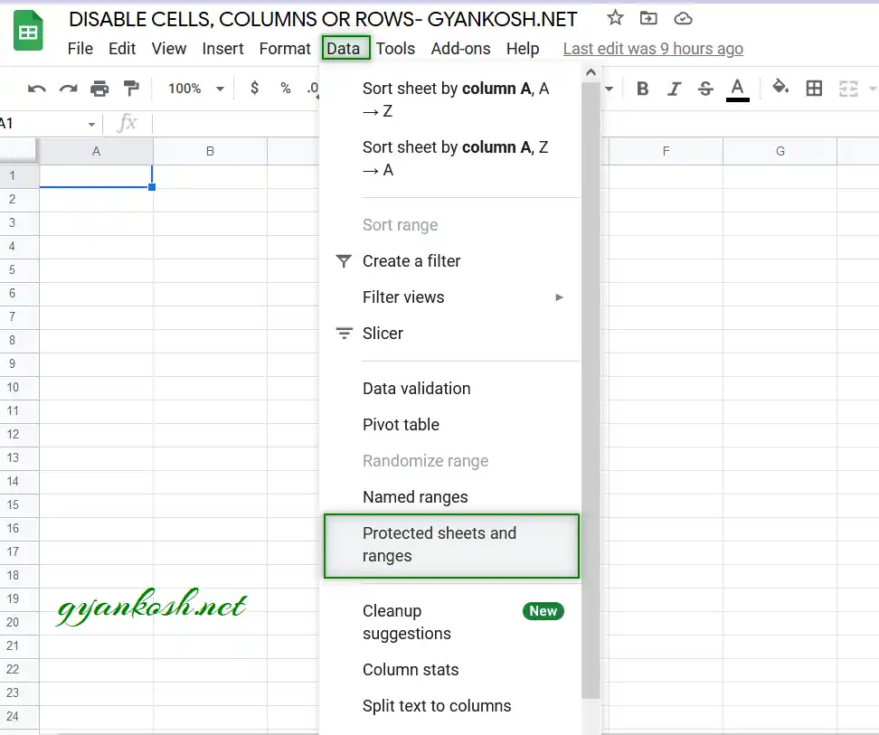
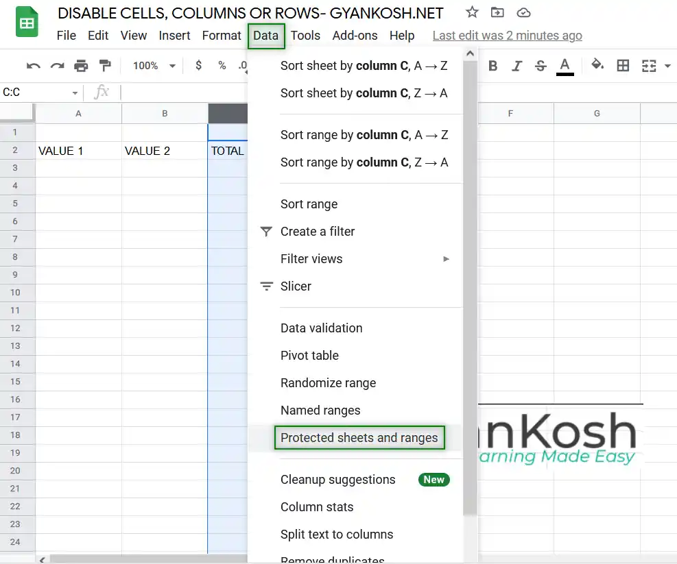
• Go to DATA MENU and choose PROTECTED SHEETS AND RANGES.

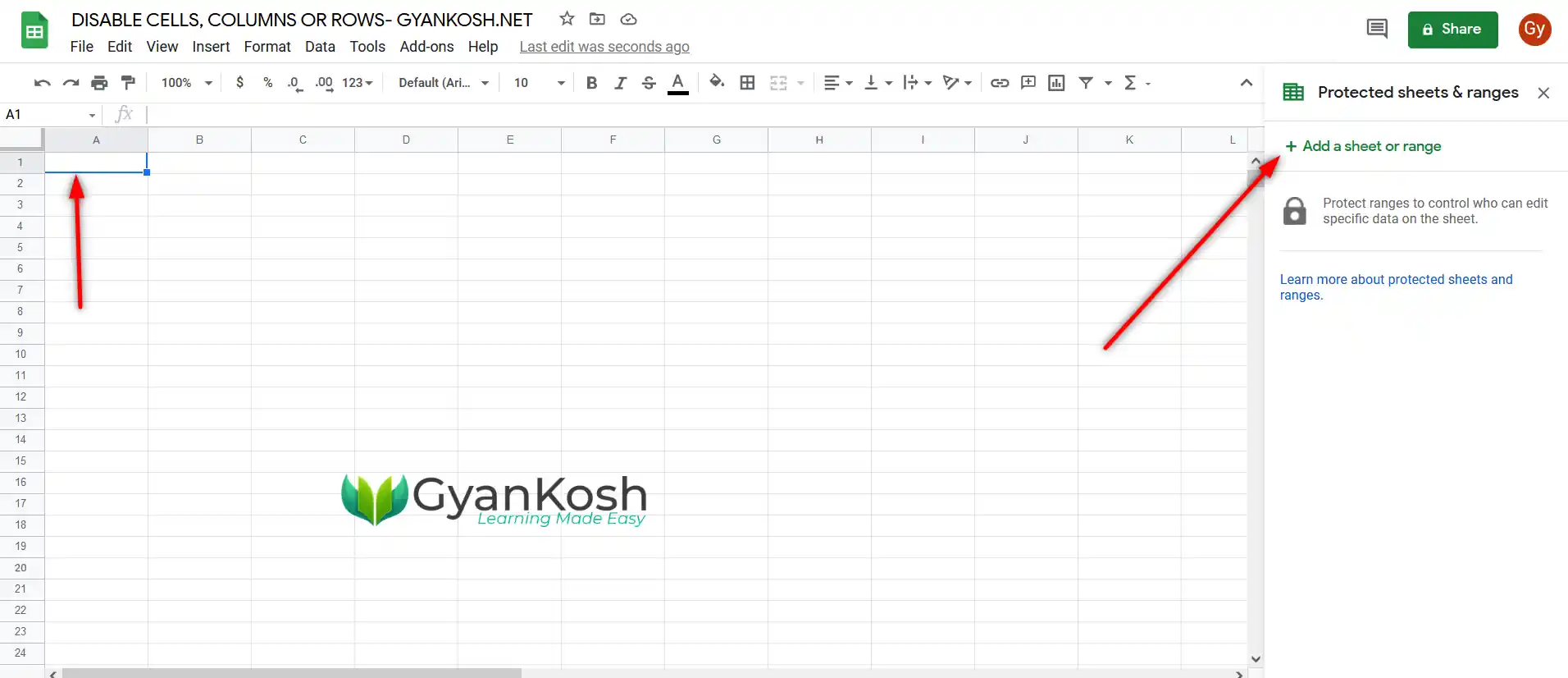
• As, we choose the option, the option box will open on the Right portion of the screen.
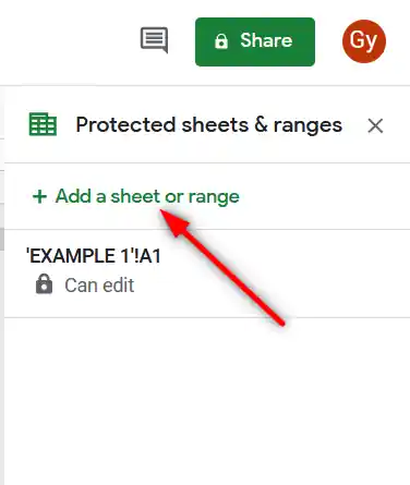
• Select the cell which you want to lock and click on ADD A SHEET & RANGES from the newly opened box as shown in the picture below.
  

• As we click ADD A SHEET OR RANGE, small dialog box will open.

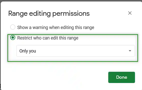
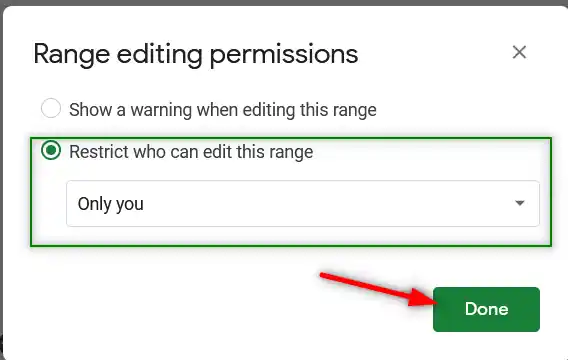
• Choose RESTRICT WHO CAN EDIT THIS RANGE and choose ONLY YOU from the drop down as shown in the picture below.

• After choosing the option, click DONE.

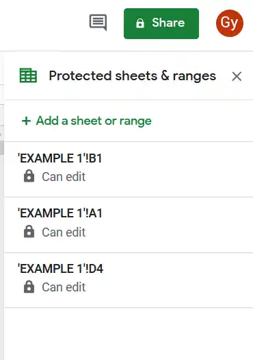
• After the rule for a cell has been set, it’ll get enlisted in the opened option box on the right portion of the screen.

• We need to disable the editing in THREE CELLS , so again click ADD A SHEET OR RANGE as shown in the picture below.

• After this, select the next cell i.e. B1 and it’ll be selected in the SELECT A RANGE, click OK.
  
  

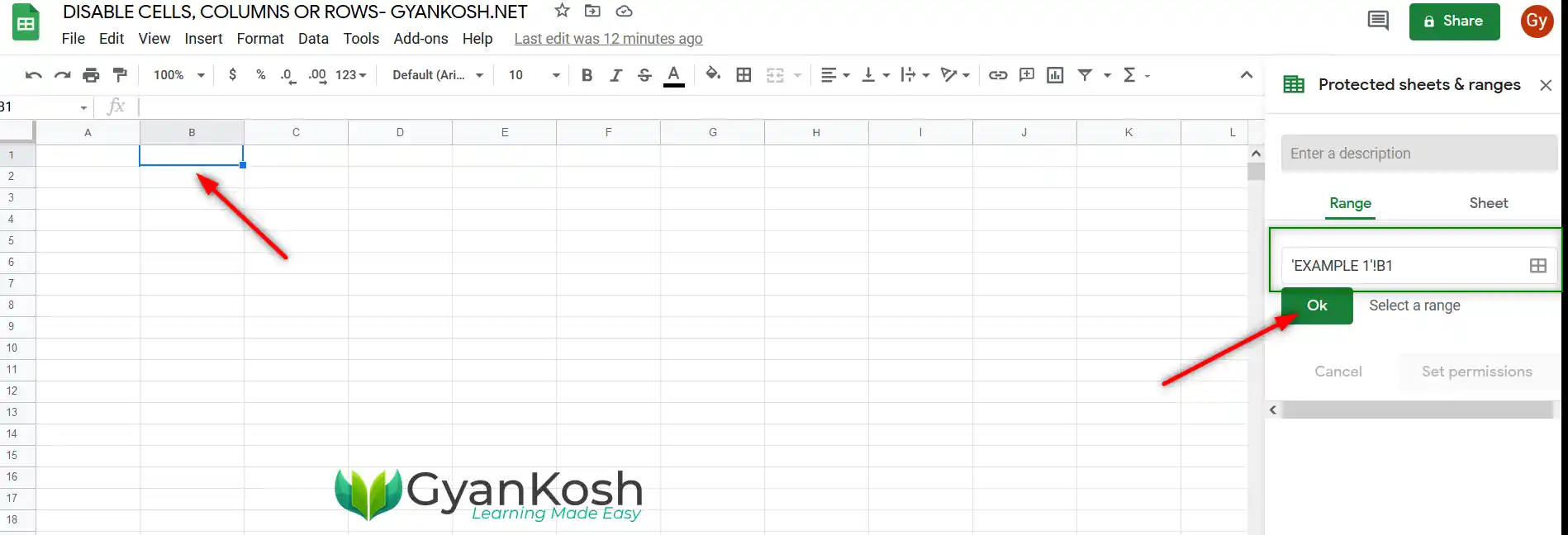
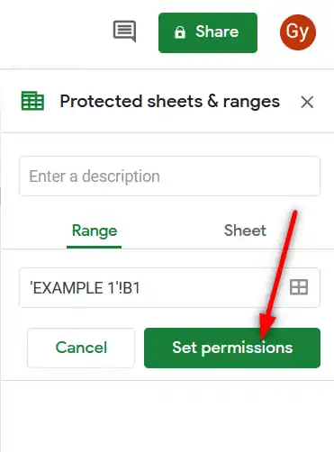
• As, the cell is finalized, click SET PERMISSION.
  

• Again choose RESTRICT WHO CAN EDIT THIS RANGE to ONLY YOU. [ It is a repeated step ].
  

• Repeat the steps for the third cell D4.

• After all the locks have been protected, the list would be something like the one shown below.
  

CHECKING THE DISABLED CELLS

Let us check the disabled cells if they are still editable or not.

• Login using any other google account.

• Share the google sheet with this new account.

• Open the sheet and try editing the disabled cells A1, B1 or D4.

• The new account won’t be able to do any changes to these cells.

• The following animation shows the process.

EXAMPLE 2: DISABLE EDITING IN COLUMN C IN GOOGLE SHEETS

SOLUTION:

We’ll use the protection option to solve this problem and disable the column C so that nobody can edit the cells in column C.

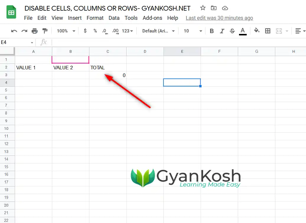
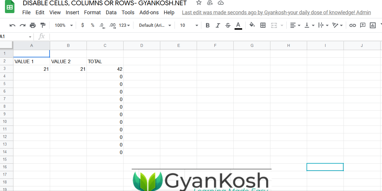
In this example, we’ll disable the COLUMN C as shown in the picture below.

We have an example where column A and column B are having two values.

Column C contains the total and we don’t want the users to make any changes in the COLUMN C.

FOLLOW THE STEPS TO DISABLE THE COLUMN C.

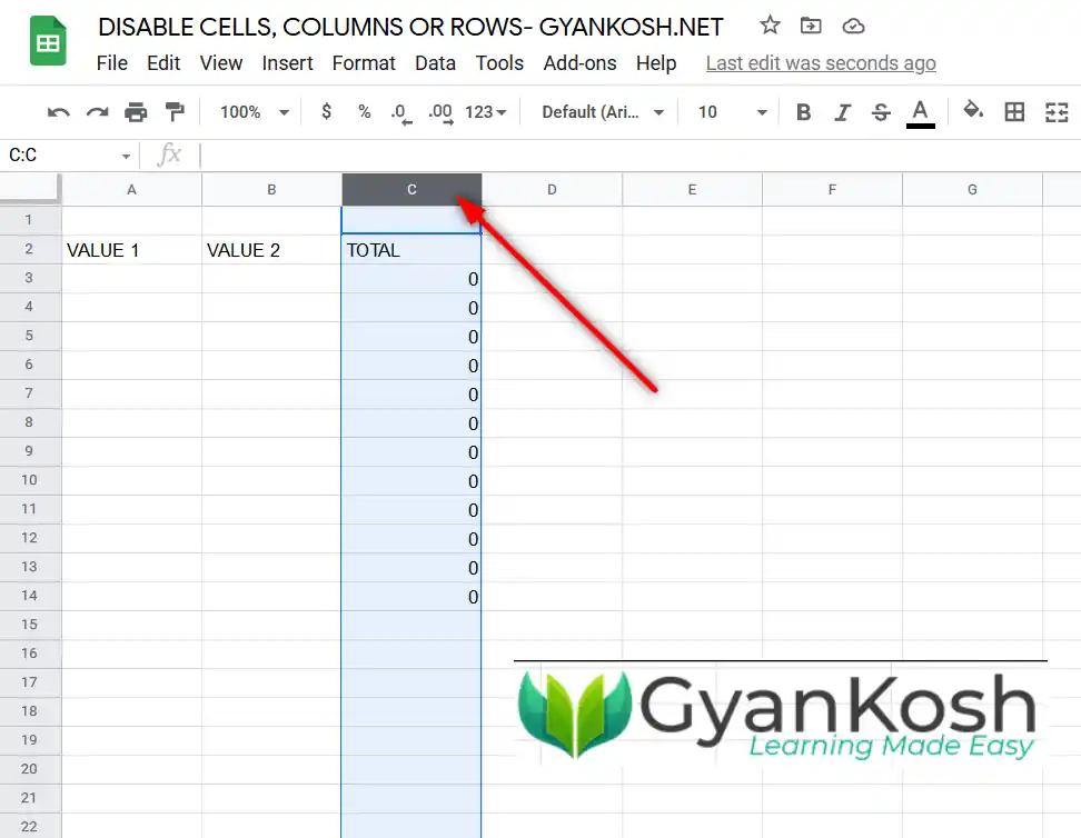
• Click COLUMN NAME C which will select the complete COLUMN C.

• Go to DATA MENU and choose PROTECTED SHEETS AND RANGES.
  

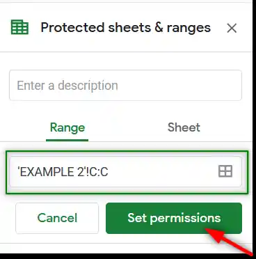
• The PROTECTED SHEETS AND RANGES option box will open on the right side.

• The COLUMN WILL BE SELECTED as we clicked the option after selecting the column.

• Click SET PERMISSIONS.
  

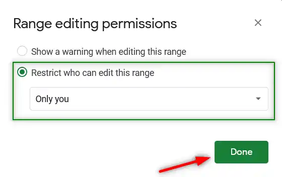
• The RANGE EDITING PERMISSIONS dialog box will open.

• Choose RESTRICT WHO CAN EDIT THIS RANGE and select ONLY YOU from the drop down.
• Click DONE.

CHECKING THE DISABLED COLUMN

Let us check the disabled column if it is still editable or not.

• Login using any other google account.

• Share the google sheet with this new account.

• Open the sheet and try editing the disabled column C.

• The other account user won’t be able to do any changes to these cells.

• The following animation shows the process.

EXAMPLE 3: DISABLE ANY EDITING IN ROW NUMBER 6

SOLUTION:

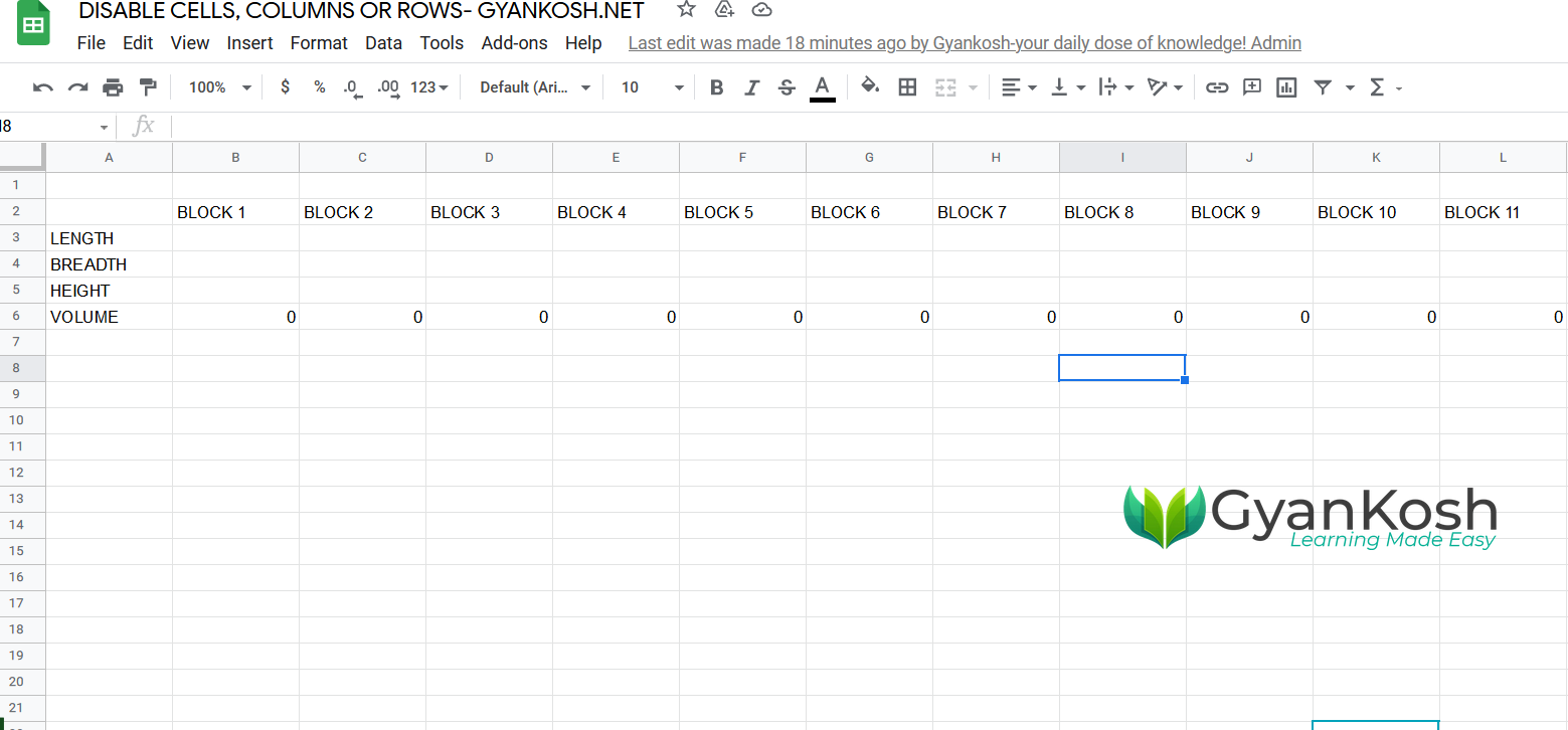
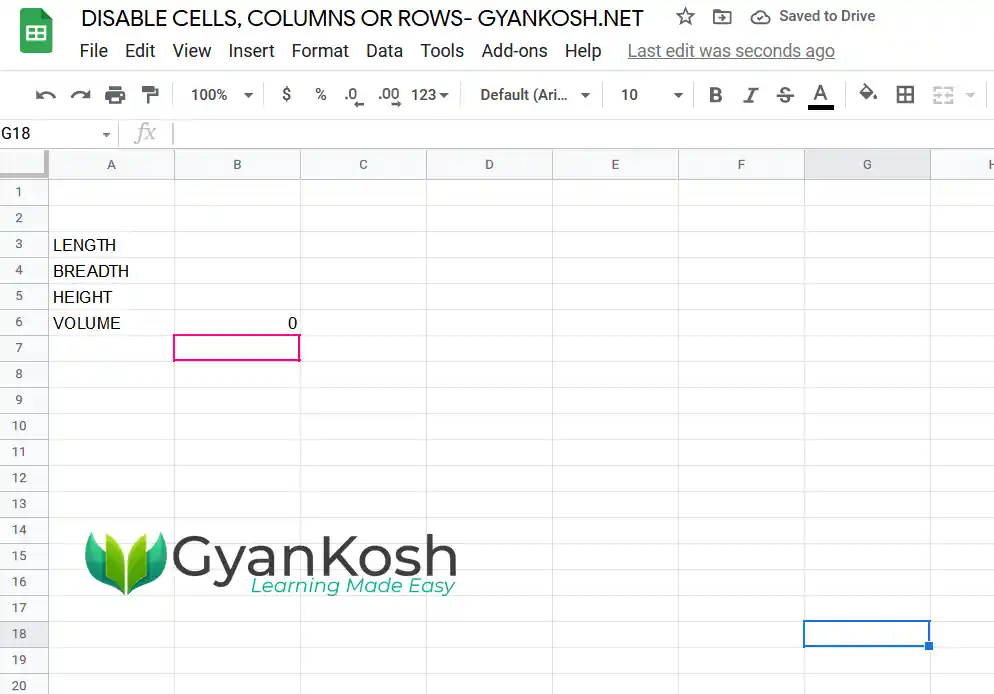
In this example, we have taken an example to find out the volume of a cubicle when length , breadth and height of the box is given.

We want the user to only be able to make changes in the LENGTH, BREADTH and HEIGHT.

We don’t want user to create any type of changes in the ROW 6 i.e. the VOLUME RESULT ROW.

The example is shown below.

FOLLOW THE STEPS TO DISABLE ROW NUMBER 6 FROM EDITING

• Select ROW 6 by simply clicking over the ROW NUMBER 6.

• Go to DATA MENU and choose PROTECTED SHEETS AND RANGES.

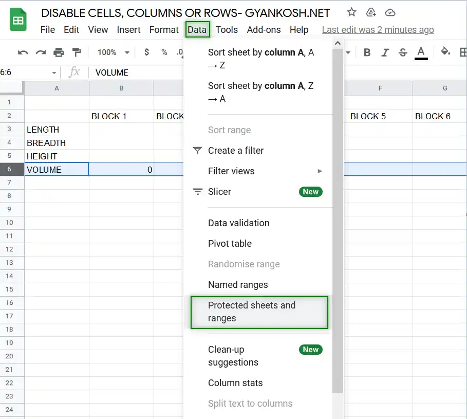
• The PROTECTED SHEETS AND RANGES OPTION BOX will open on the right.

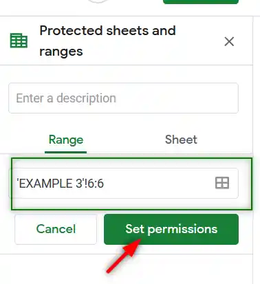
• As , we had already selected the row before choosing the option, RANGE WILL APPEAR FIELD CORRECTLY.

• Click SET PERMISSIONS.

• As we click SET PERMISSIONS, the following dialog box will open.

• Choose RESTRICT WHO CAN EDIT THIS RANGE and ONLY YOU from the drop down.
• Click DONE.

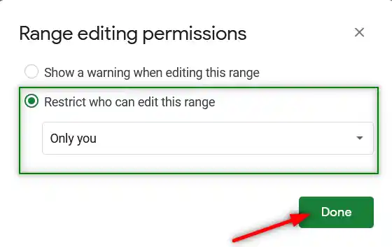
The row has been disabled and can’t be edited by the users.

CHECKING THE DISABLED ROW

Let us check the disabled row if it is still editable or not.

• Login using any other google account.

• Share the google sheet with this new account.

• Open the sheet and try editing the ROW 6.

• The other user account won’t be able to do any changes to these cells.

• The following animation shows the process.