PROVIDING ACCURATE, RELIABLE AND STRAIGHT TO THE POINT KNOWLEDGE ABOUT DIFFERENT IT TOOLS EXPLAINED WITH PRACTICAL EXAMPLES

how to lock OR UNLOCK cells in google sheets ?

INTRODUCTION

GOOGLE SHEETS has many great features. One of these great features is its Sharing Capabilities which gives us a very smooth experience when we share our sheets with somebody and when we decide the permissions to edit, or just view as per our discretion.

LOCKING OR PROTECTING CELLS OR SHEETS IN GOOGLE SHEETS MEAN TO LIMIT THE ACCESS TO EDIT THE DATA IN PARTICULAR CELLS OR SHEETS. WE CAN ALSO LIMIT THE EDITING TO FEW SPECIFIC PEOPLE.

In this article we will learn the way to lock or protect a particular group of cells, permit a few people to edit the cell, show the warning while editing and more options available in google sheets.

HOW TO LOCK CELLS IN GOOGLE SHEETS

Let us first learn to lock the cells in google sheets.

Its always a great habit to learn with practical. So, let us take an example and learn the process of locking the cells from editing.

Let us assume a fictitious data in our sheet.

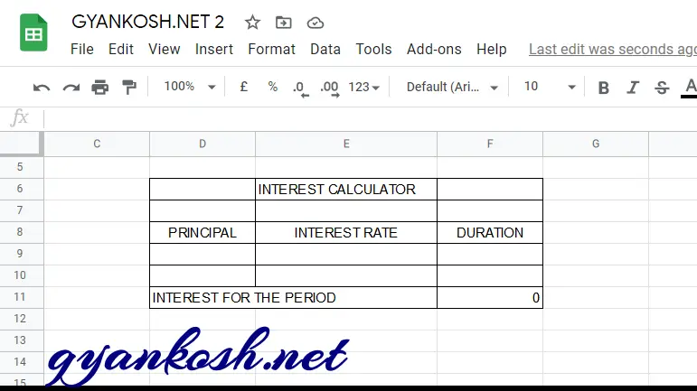
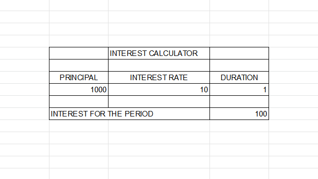
We have created a SIMPLE INTEREST CALCULATOR.

We don’t want the user to edit the result cell which contains the formula. So we’ll try to lock this cell to avoid any change in the cell by mistake.

	INTEREST CALCULATOR

PRINCIPAL	INTEREST RATE	DURATION


INTEREST FOR THE PERIOD		0

Let us put the values in the calculator and check the result.

	INTEREST CALCULATOR

PRINCIPAL	INTEREST RATE	DURATION
1000	10	1

INTEREST FOR THE PERIOD		100

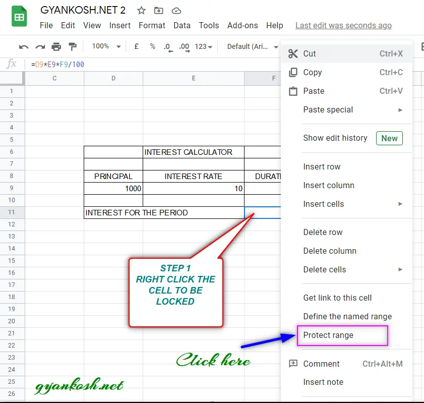
STEPS TO LOCK CELL IN GOOGLE SHEETS:

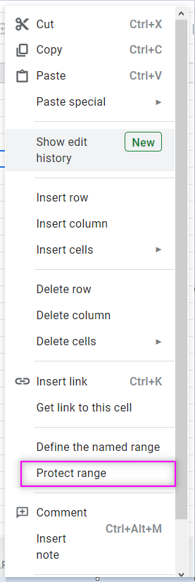
Right Click the cell or range which you want to lock or protect.
Select PROTECT RANGE.

The picture below shows the button locations.

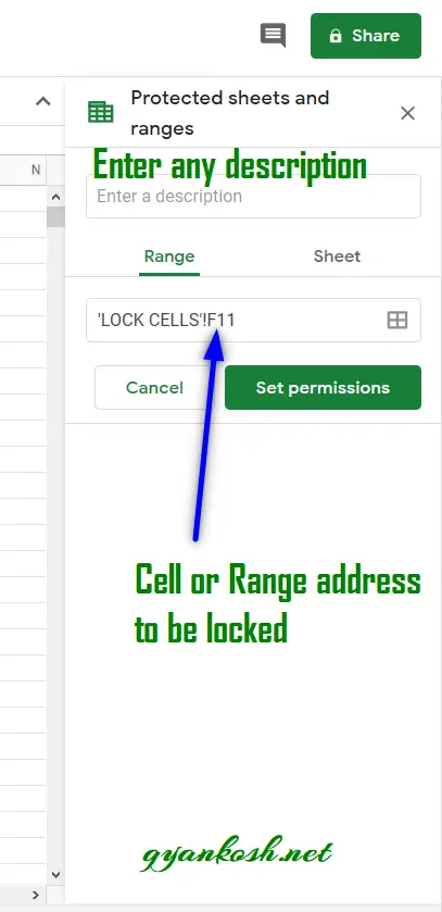
The PROTECTED SHEETS AND RANGES option box will appear on the right side of the Google Sheets.
As we have already selected the Cell, it’ll appear in the RANGE FIELD as shown in the picture below.
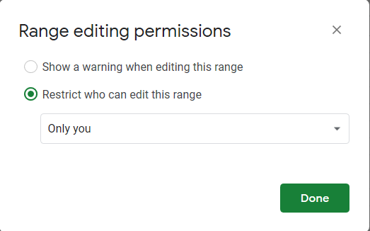
Click SET PERMISSIONS.

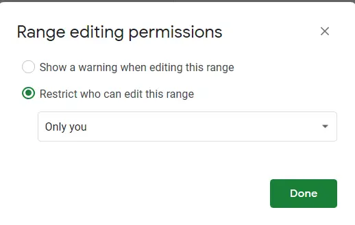
A small dialog box will open for editing the Range Permissions.
From the RESTRICT WHO CAN EDIT THIS RANGE, select ONLY YOU.
It’ll lock this cell for everybody else.
Look at the picture below for reference.

The cell containing the simple interest is locked for everybody else.

THE PROTECTION SYSTEM IN GOOGLE SHEETS IS A BIT DIFFERENT FROM THE MICROSOFT EXCEL. MICROSOFT EXCEL GIVES US OPTION TO APPLY PASSWORDS BUT GOOGLE SHEETS WORKS ON THE BASIS OF THE GOOGLE ACCOUNT LOGIN AND CONTROLLING THE ACCESS OF DIFFERENT USERS.

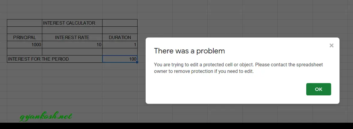
We shared this sheet with another user and tried changing the locked cell.

The Google Sheets returned an error.

Look at the picture below.

HOW TO PROTECT COMPLETE SHEET IN GOOGLE SHEETS

In the previous section, we learnt to lock a single cell or group of cells .

Now, let us learn to lock a complete SHEET from being edited by anybody.

STEPS TO LOCK A COMPLETE SHEET :

Right Click on the Sheet anywhere. [ The sheet which we want to protect or lock ].

Now the PROTECTED SHEETS AND RANGES DIALOG BOX will open on the right.

Carefully click the SHEETS TAB as we want to lock the sheets this time.

Choose the sheet from the drop down. [THE DROP DOWN CONTAINS ALL THE SHEETS IN YOUR WORKBOOK ]
By default, the selected sheet will be the one from which we started the process. The sheet we’re working was LOCK CELLS.
It can be seen in the picture below.
After selecting the sheet , click SET PERMISSIONS.

A small RANGE EDITING PERMISSIONS dialog box will open.
Choose RESTRICT WHO CAN EDIT THIS RANGE radio button and ONLY YOU from the drop down as shown in the picture below.
Click DONE.

The SHEET IS LOCKED FROM EDITING.

Let us check the sheet.

The sheet can’t be edited at all. All the contents can just be viewed only.

ACCESS CONTROL FOR LOCKED CELLS OR LOCKED SHEETS IN GOOGLE SHEETS

Till now , we learnt the ways to lock a few cells or complete sheet in google sheets.

Let us now check how we can authorize a few selected users to be able to edit the data.

Let us lock the complete INTEREST CALCULATOR and then share its editing authorizations with other selected users.

FOLLOW THE STEPS TO LOCK THE COMPLETE INTEREST CALCULATOR

[ Already, complete description has been given for locking the cells , so we’ll discuss it in brief only ].

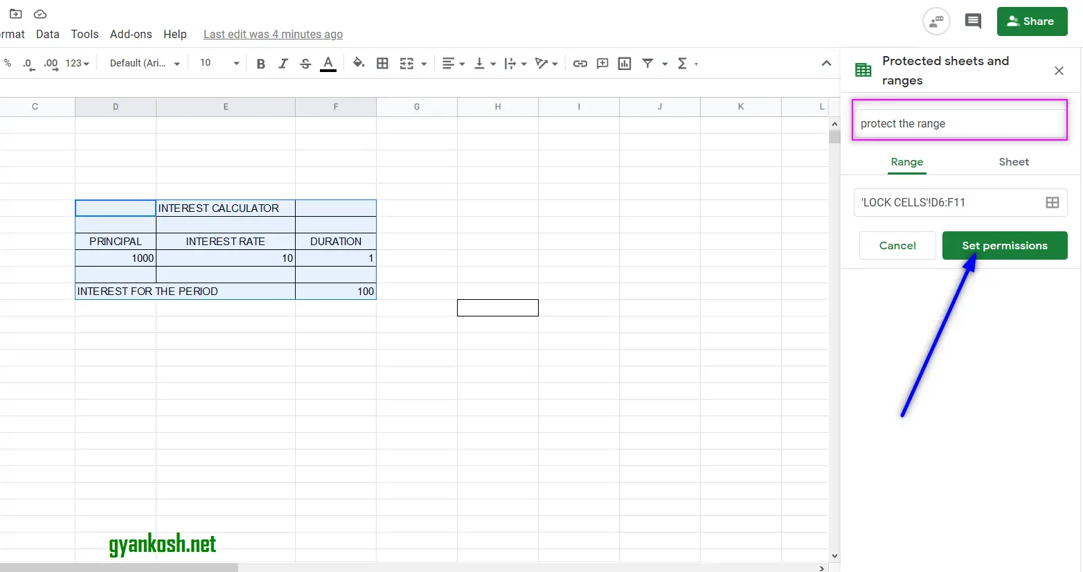
Select all the cells of INTEREST CALCULATOR.
Right Click and choose PROTECT RANGE.
Enter any description.
Check the Range if it is correct and click SET PERMISSIONS.

As we click SET PERMISSION, a small window will open asking about the permissions.
Yes, we are acquainted with this window but this time, we’ll use other option.
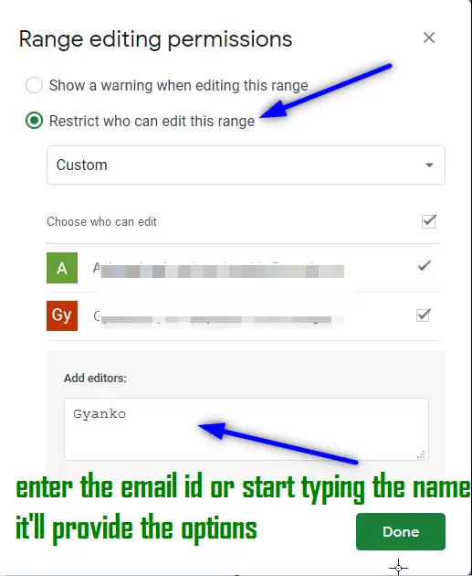
Select RESTRICT WHO CAN EDIT THIS RANGE radio button as marked in the picture below.
Select CUSTOM from the drop down.
As we select custom, we’ll get a list of the opened accounts, as shown in the picture below as A and Gy, obfuscated for privacy reason.
We can choose the users from there if the intended users are listed.
If not, reach ADD EDITORS in the bottom of the window, and add the Name or the email ID of the user.
As we start typing the name, google sheets will start offering the suggestions and we can choose from them.
After adding the editors, click DONE.

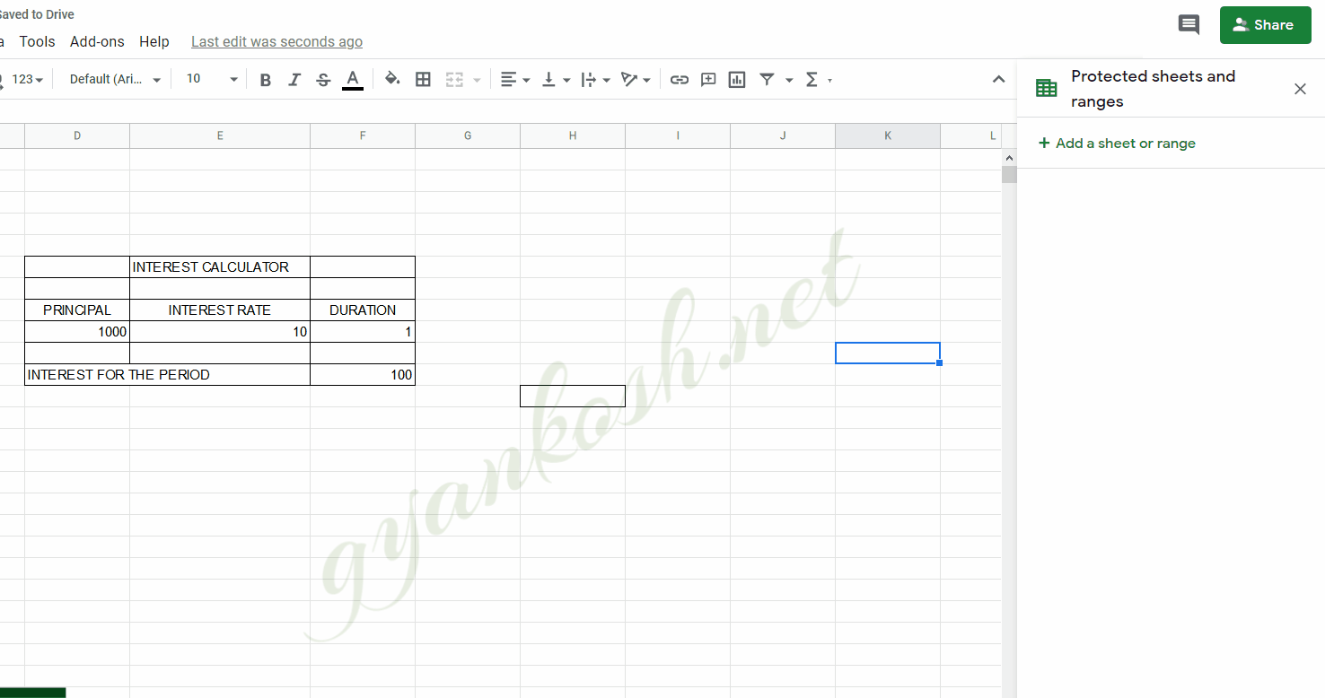
After clicking DONE, we are done with the limited access to our cells or sheets where the users who are granted access will be able to make the changes to the cells or sheets.

SHOW A WARNING MESSAGE BUT ALLOW EDITING OF CELLS

Out of the many useful options, the last option is to show a warning message when you try to edit the cells but allowing the editing.

Let us learn to lock cells such that they just show a warning message when somebody tries to change the cells.

STEPS TO ADD A WARNING MESSAGE BUT ALLOW EDITING OF CELLS:

Select the group of cell or the Sheet which you want to lock or protect.
Right Click and choose PROTECT RANGE.
The protected Sheet and Range options dialog box will appear on the Right.

After we click SET PERMISSIONS a small dialog box will enter.
Choose the RADIO BUTTON bearing SHOW A WARNING WHEN EDITING THIS RANGE caption.
Click DONE.
Now when somebody tries to make some change in the cells or the sheet, a warning message will be displayed.

HOW TO UNLOCK LOCKED CELLS IN GOOGLE SHEETS ?

In the previous sections we learnt about many ways to protect the cells or sheets.

Now, at the end, let us learn to unprotect or unlock the locked cells or a sheet in google sheets.

FOLLOW THE STEPS TO UNLOCK LOCKED CELLS IN GOOGLE SHEETS.

Right Click the locked cells or locked sheet.
Go to PROTECT SHEET.

It’ll open the PROTECTED SHEET AND RANGES DIALOG BOX.
The dialog box will enlist all the protection rules applied on the selected cells or sheets.
Click the locking or protection rule.

Click on the DELETE button adjacent to the top field of DESCRIPTION and the rule will be removed.

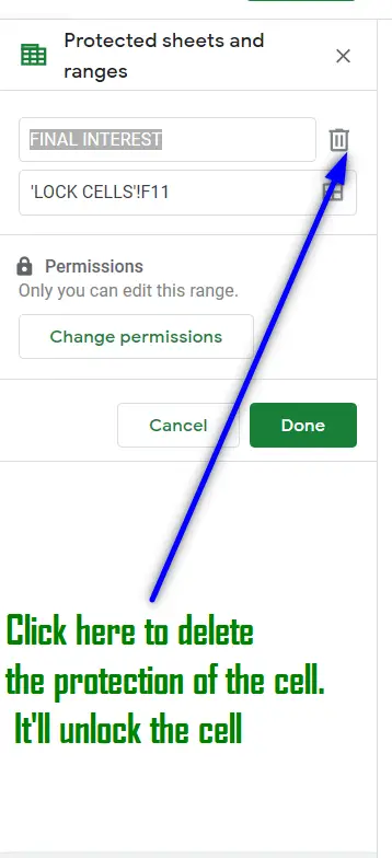
Click DONE.
The locking has been removed.

Contents