Table of Contents
- INTRODUCTION
- HOW HOURS ARE HANDLED IN GOOGLE SHEETS?
- ADD HOURS IN GOOGLE SHEETS
- HOW TO EXTRACT THE HOURS FROM THE GIVEN TIME IN GOOGLE SHEETS ?
- HOW TO ADD HOURS TO THE GIVEN TIME
- ADD HOURS TO HOURS IN GOOGLE SHEETS
- ADD HOURS AND RESULT SHOULD BE IN HOURS ONLY
INTRODUCTION
Google Sheets is emerging as a good options for spreadsheets usage.
Spreadsheets are used for making our jobs simpler by creating the automated reports by using functions, formats and many other options present in the Google Sheets.
But some of the features can become confusing for some naive users. One such feature is the handling of the time in google sheets.
On one side, it makes it very easier for us to handle time in google sheets, once it starts creating problems, it becomes almost impossible to handle unless you have very clear concepts regarding the time handling in Google Sheets.
In this article, we’ll particularly focus about handling the hours [ from the time] in various ways.
HOW HOURS ARE HANDLED IN GOOGLE SHEETS?
Time and date go side by side.
Date is taken as a number starting from Dec 31,1899 whereas time is taken as the decimal part of the same.
1 is divided by the total number of seconds i.e. 1/86400. The decimal result will represent the 1 second.
Multiplying this value with 3600 [ i.e. the number of seconds in an hour ] the value comes out to be 0.04166666667.
It means, if we type 0.04166666667 in the cell and change the format to TIME, it’ll get converted to 1 AM.
In this article, we’d try out different ways of handling the HOURS in Google Sheets.
ADD HOURS IN GOOGLE SHEETS
Let us learn the way to add hours in Google Sheets.
Adding the hours will create different scenarios which can be simple or complex.
- Adding Hours to the Time
- Adding Hours to the Hours
- Adding hours with result in Hours only
We’ll discuss these three scenarios which come across frequently whenever we try to handle time in google sheets.
But before that we should know the way to extract hours from the time which might be needed in some cases.
HOW TO EXTRACT THE HOURS FROM THE GIVEN TIME IN GOOGLE SHEETS ?
The time format is given by the standard HOUR:MINUTES:SECONDS form. There are different formats which we can choose from the options available.
There is a dedicated function to help us extract the HOURS from the given time in any format.
ALWAYS REMEMBER! FORMAT IS JUST A PRESENTATION. IN THE BACK END , THE VALUES ARE THE SAME IN DIFFERENT FORMATS. SO THE APPLICATION OF ANY FUNCTION ON THE DIFFERENT FORMATS WILL RESULT IN THE SAME RESULT.
FOLLOW THE STEPS TO EXTRACT HOURS FROM THE GIVEN TIME:
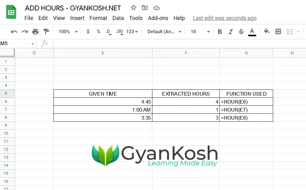
- Double click the cell where you want the result as HOURS extracted from the given time.
- Enter the formula as =HOUR(CELL CONTAINING TIME/ TIME INSIDE DOUBLE QUOTES).
- Press ENTER.
- The result will appear as the HOURS in the time.
HOW TO ADD HOURS TO THE GIVEN TIME
In this case, we are going to add hours to the given Time. [ TIME FORMAT]
For example if we want to add 3 hrs to any given time for creating slots, or any schedules etc.
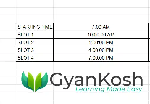
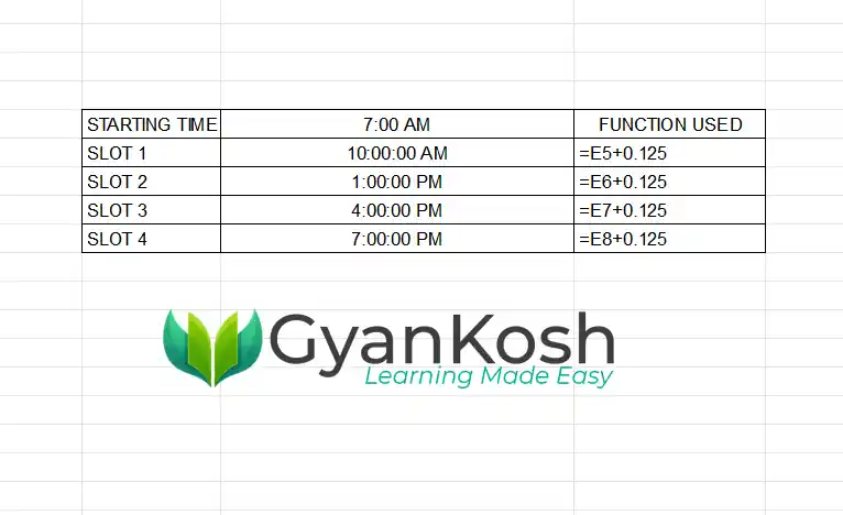
To learn this, let us create a template with three hours slot.
We’ll change the basic time and the slots will change automatically.
The situation is something like as shown in the picture below.
We can add the hours in two different ways to the given time.
- Adding the hours directly. [ As shown in the picture above ].
- Adding the hours by taking them in the different cell or cells and then adding them. [ As shown in the picture below ]
We’ll discuss both the ways one by one.
WAY 1: ADDING HOURS TO THE GIVEN TIME
SOLUTION:
We can see in the sample picture above that we have directly added the hours to the time given in one cell and the result is correct.
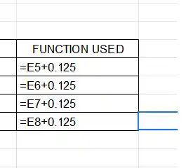
But look at the formula used.
You can see that the formula used is CELL CONTAINING THE TIME+0.125
WE CAN'T SIMPLY ADD HOURS TO THE CELL CONTAINING THE TIME E.G. =15:00+3:00 WILL CAUSE AN ERROR AND IS AN INVALID PROCEDURE.
For the correct procedure, we need to derive the numerical value of the 3 hours and then add it to the cell.
The result will appear. If the result is absurd, change the format to time and you can have the correct result in the correct format.
CALCULATING THE NUMERICAL VALUE FOR THE GIVEN HOURS
As we already discussed in the previous sections 1 hr=0.0416666667
Multiply the numerical value by 3.
The result is 0.125 which is the value we added.
The result will appear as the time after three hours simply.
FOLLOW THE STEPS TO ADD HOURS TO THE GIVEN TIME BY ADDING THE HOUR DIRECTLY TO THE TIME
- The first step is to find out the numerical value of the HOURS , you want to add to the given time. [ Simply multiply the number of hours by 0.04166667 ]
- Double click the cell where you want the result.
- Enter the formula as =CELL CONTAINING THE TIME+ NUMERICAL VALUE EMERGED FROM THE CALCULATION OF HOURS.
- For our example the formula will become =E5+0.125.
- Press ENTER.
- The result will appear as the time after 3 hours from the starting time.
- Drag down the formula and it’ll add 3 hours to the time appearing on the left and will help us create the slots.
WAY 2: ADDING THE HOURS SEPARATELY IN THE CELLS
This is an easier way of adding the hours to the given time.
In this style, we simply put the hours in the separate cells and add it to the already given time in another cell.
No issues will emerge in this style except that we do need an extra column or cell.
The result will appear as the time after three hours simply.
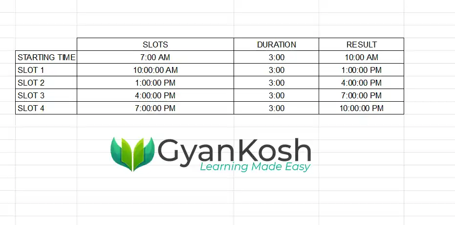
The following picture shows the way which can be used to add the hours simply to the given time.
FOLLOW THE STEPS TO ADD HOURS TO THE GIVEN TIME USING EXTRA COLUMN.
- Create an extra column to enter the hours to be added.
- Double click the cell where you want the result to appear.
- Enter the formula as =cell containing the time + cell containing the time to be added.
- For our example, the formula will be
- Press ENTER.
- The result will appear as the HOURS in the time.
ADD HOURS TO HOURS IN GOOGLE SHEETS
Another case arises in the Google Sheets when we want to add the HOURS to the HOURS.
This is also one of the most frequent cases which are required to be dealt properly and carefully.
Although the solution is pretty simple but we need to be careful about a few things.
PER-REQUISITIONS FOR THE DATA:
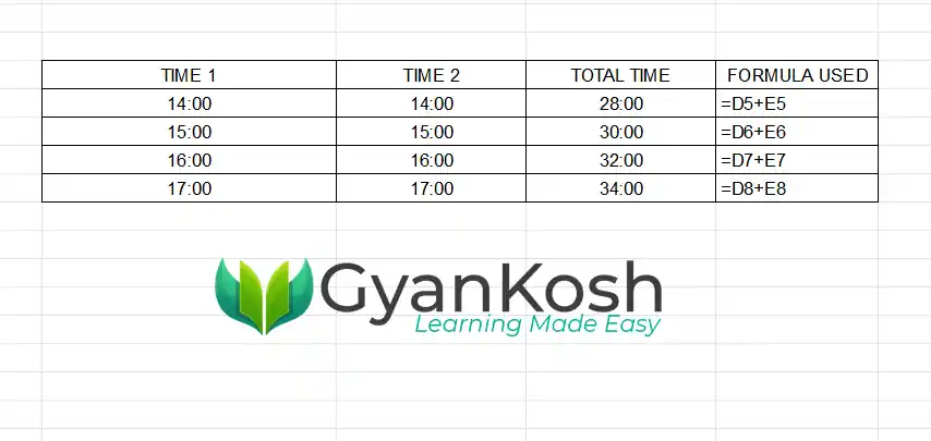
The data needs to be in the different columns. The picture below shows the data under the heading TIME 1 and TIME 2.
We’ll find out the sum of the given hours in both the columns.
FOLLOW THE STEPS TO ADD THE HOURS TO THE HOURS IN GOOGLE SHEETS
- Double click the cell where you want the result to appear.
- Enter the formula as =cell containing the first time + cell containing the second time.
- For our example, the formula will be =D6+E6 for the first line in ROW 6.
- Press ENTER.
- The result will appear as the TOTAL HOURS in the COLUMN F.
- Drag down the formula to get the result of the rest of the cases.
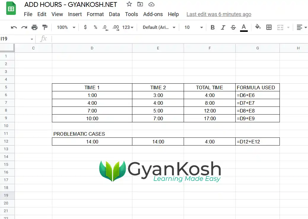
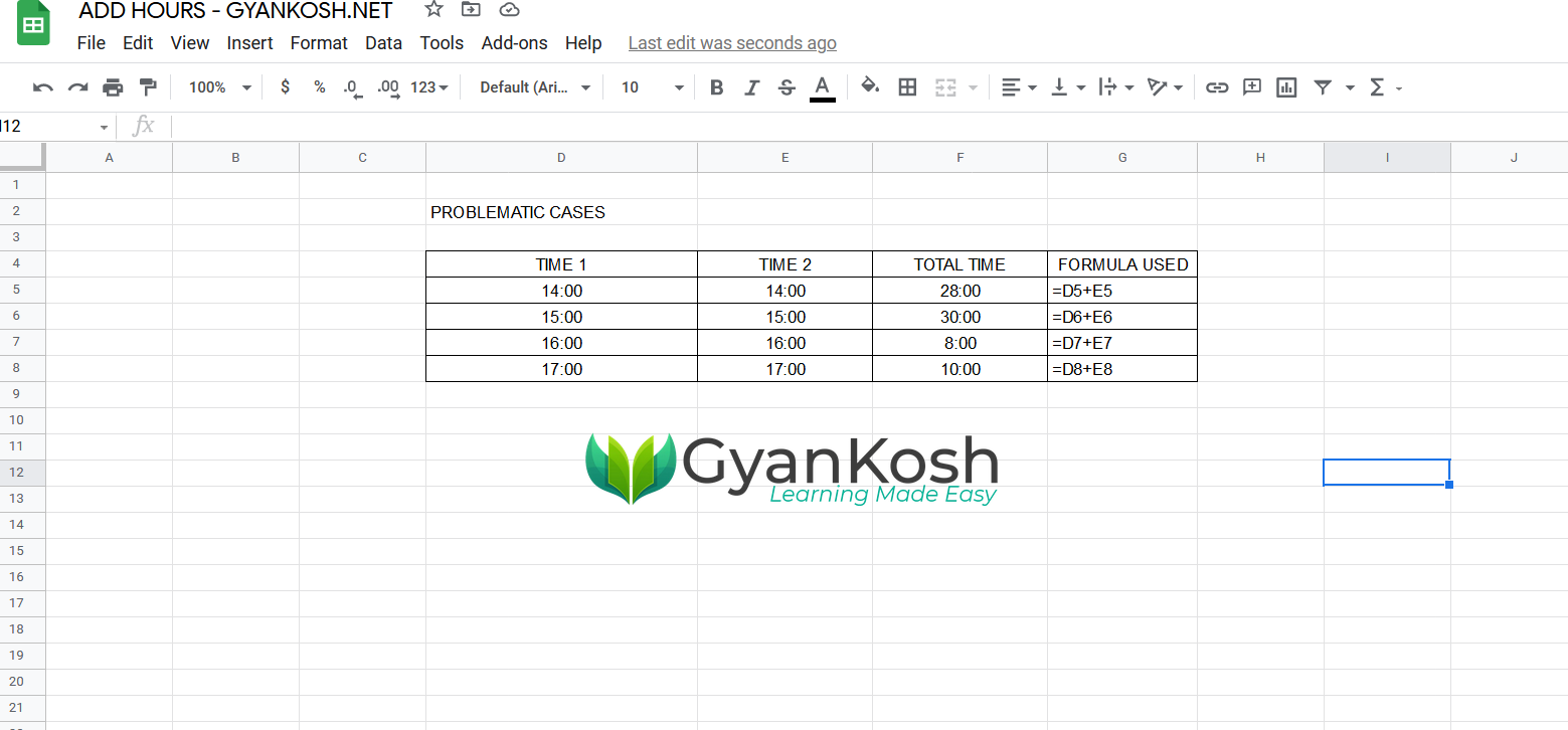
CAUTION: This method is very simple but it’ll sum up the total number of hours up to 24 hours only.
Have a look at the picture above and ROW NO. 12
ADD HOURS AND RESULT SHOULD BE IN HOURS ONLY
This is the third case where we’ll add hours to the hours but we want the result as the total hours only and no changes in the date.
For this, we’ll use the second way only but we’ll change the format of the resulting cell so that it shows the total hours without any date change.
FOLLOW THE STEPS TO ADD HOURS TO THE GIVEN HOURS OR TIME WITH THE RESULT AS TOTAL HOURS
- After we have added the time in the standard way as discussed here.
- Select the RESULT CELL [ where we want to change the format of the cell to show the net total hours ].
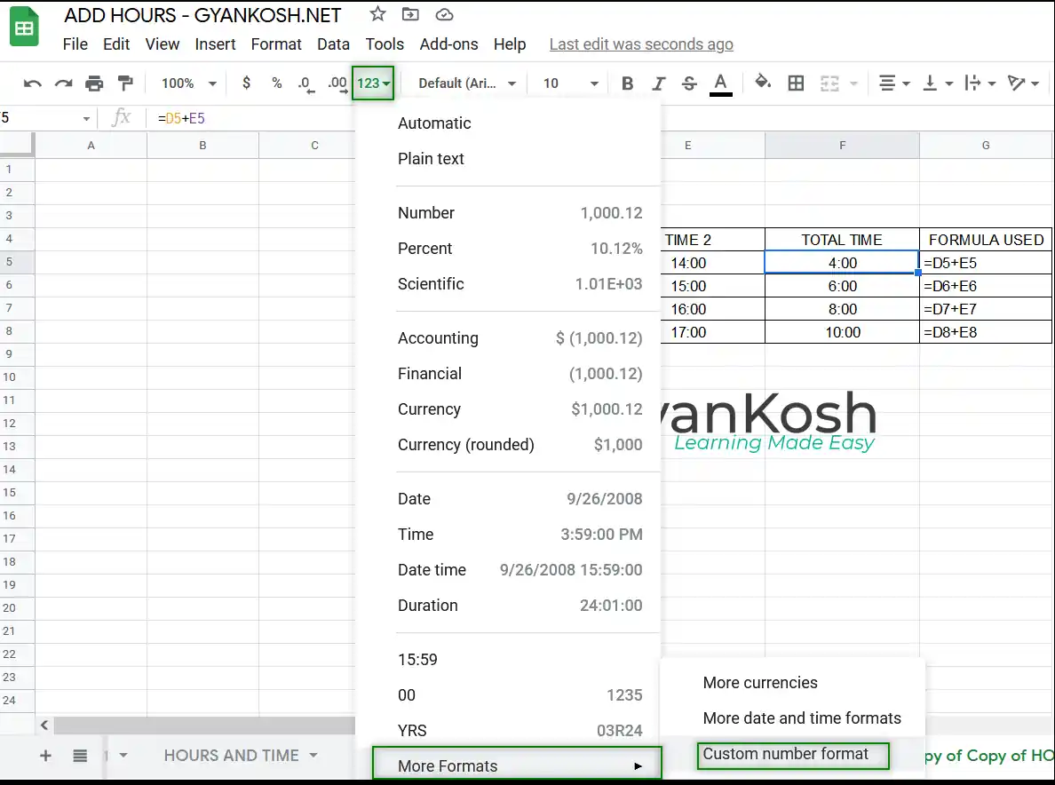
- Go to FORMAT CHANGE > MORE FORMATS > CUSTOM NUMBER FORMAT.
- The location is shown below in the picture.
- As we choose CUSTOM NUMBER FORMAT, the following window will open.
- In the custom format type [H]:MM or [h]:mm.
This format is telling GOOGLE SHEETS to show the total hours and minutes only.
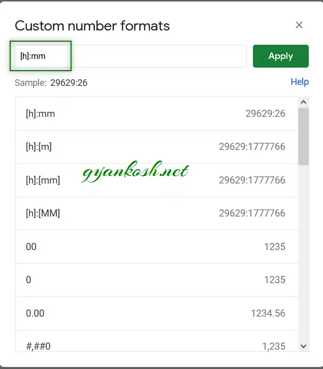
- After inserting the format as mentioned above, click Apply.
- The result will simply change to the total hours.
ONCE YOU HAVE SET THE FORMAT FOR ONCE CELL, THERE IS NO NEED TO REPEAT THIS PROCEDURE FOR ALL THE CELLS. FOLLOW THE PROCEDURE.
COPYING THE FORMAT TO OTHER CELLS
There is a dedicated functionality known as PAINT FORMAT in Google Sheets for copying the format. This function not only copies the color, fonts etc. but formatting rules too.
CLICK HERE TO LEARN DETAILED PAINT FORMAT USAGE.
FOLLOW THE STEPS TO COPY THE FORMAT FROM ONE CELL TO ANOTHER.
- Select the cell whose format needs to be copied.
- Click PAINT FORMAT.
- Select the cell where you want to paste the format.
- The formatting of the destination cell will be changed as per the original cell.
- The complete process is shown in the picture below.
- After making all the changes, we can see that we got the results corrected.
- The following picture shows all the results.