Table of Contents
- INTRODUCTION
- WHAT IS CONDITIONAL FORMATTING BASED ON CHECKBOX?
- EXAMPLES:
- EXAMPLE 1: HIGHLIGHT THE CELLS BY CHECKING OR UNCHECKING THE CHECKBOX
- EXAMPLE 2: HIGHLIGHT THE COMPLETE ROW BY CONDITIONAL FORMATTING USING CHECKBOX CONTROL
- EXAMPLE 3: HIGHLIGHT THE COMPLETE COLUMN BY CONDITIONAL FORMATTING USING CHECKBOX CONTROL
- FAQs
- HOW TO CHANGE THE COLOR OF THE CHECKBOX IN GOOGLE SHEETS?
INTRODUCTION
Whenever we prepare any report in GOOGLE SHEETS, we have two constituents in any report.
The Text portion and the Numerical portion.
But just storing the text and numbers doesn’t make the super reports. Many times we need to automate the process in the reports to minimize the effort and improve the accuracy.
Conditional Formatting is a great tool offered by Google Sheets which help us highlight the useful data using the different format settings.
We can highlight the data using conditional formatting on the basis of text values, numerical values, any other conditions on text or numerical values , checkboxes etc.
We already learnt the conditional formatting on the basis of text , on the basis of another cell.
In this article we’ll learn the way to handle conditional formatting on the basis of checkbox in Google Sheets.
Let us start !
WHAT IS CONDITIONAL FORMATTING BASED ON CHECKBOX?
CONDITIONAL FORMATTING is FORMATTING BASED ON THE CONDITIONS.
Now, in this particular case, the condition will be on the state of the checkbox i.e. if it is selected or not.
It means, we’ll change the formatting of the resulting data on the basis of checkbox , if it is checked or not.
Such a situation may arise where we need to use the checkbox in our sheet and highlight the data on the basis of the checkbox state. For example, if we have various categories , we can highlight any word on the basis of the selection of the checkbox.
We’ll learn this with the help of an example.
Formatting is the APPEARANCE BASED FEATURES such as font, fill color, font color , text size etc.
The data will be highlighted using the chosen format, if the checkbox is checked and won’t be highlighted if the checkbox is not checked.
If you want to learn the basics of the conditional formatting , kindly go through the link LEARN TO USE CONDITIONAL FORMATTING IN GOOGLE SHEETS .
You’ll be amazed to see the capability of conditional formatting and its use which is awesome.
EXAMPLES:
EXAMPLE 1: HIGHLIGHT THE CELLS BY CHECKING OR UNCHECKING THE CHECKBOX
In this example, we’ll highlight cells containing specific words if checkbox is checked i.e. selected.
Let us specify the example a bit more so that we can use this example and learn the way to use Conditional formatting with checkbox.
We have created a sample data with random words and some repetition.
| HELLO | WHY |
| FUN | WHEN |
| HOW | WHAT |
| WHAT | WHY |
| HELLO | WHEN |
| HOW | YES |
| WHY | FUN |
| HELLO | WHEN |
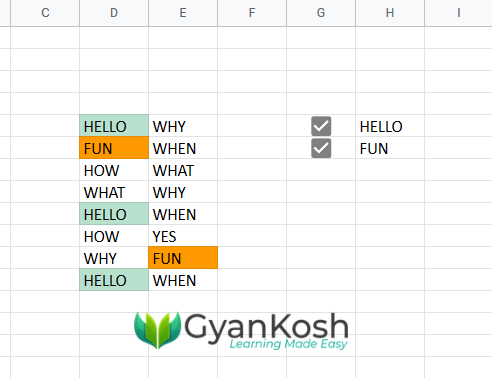
We want to highlight the chosen word from this group of words.
It’ll be like the picture shown below.
FOLLOW THE STEPS TO APPLY CONDITIONAL FORMATTING ON THE BASIS OF CHECKBOX
- For the data creation, insert the CHECKBOX in GOOGLE SHEETS as shown in the picture below.

The details [HELLO and FUN] are written in the adjacent cells.
- Rest of the data is the simple text which you can put in a table or place it in any layout as per requirement.
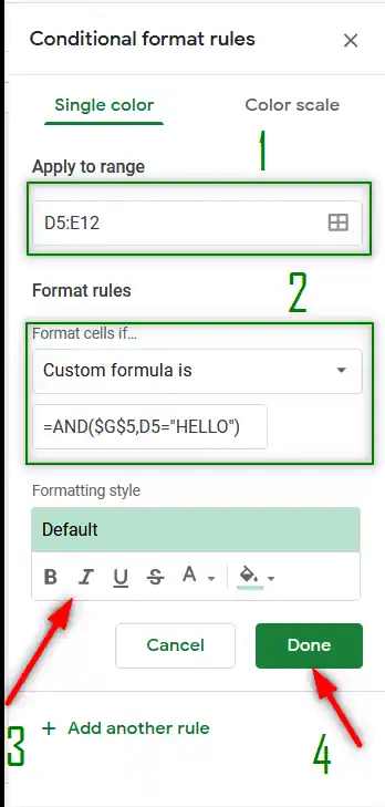
- Select the data. [Our data lies between D5 and E12 ]
- Go to FORMAT menu and choose CONDITIONAL FORMATTING.
- The CONDITIONAL FORMATTING window will open on the right.
- [1] shows the range on which we want to apply the conditional formatting.
- After setting the Range, choose CUSTOM FORMULA from the FORMAT RULES DROP DOWN [ 2 in picture ].
- Enter the formula as =AND($G$5,D5=”HELLO”).
- Set the format as per your requirement. We have kept the green fill color. [3]
- Click DONE. [4]
The following picture shows the steps.
- After the first rule has been applied, click ADD MORE RULE in the CONDITIONAL FORMATTING dialog box which can be again brought by going to FORMAT MENU
- and choosing CONDITIONAL FORMATTING.
WE NEED TO APPLY MULTIPLE CONDITIONAL FORMATTING RULES ON THE SAME DATA. [ TWICE IN THIS EXAMPLE ]
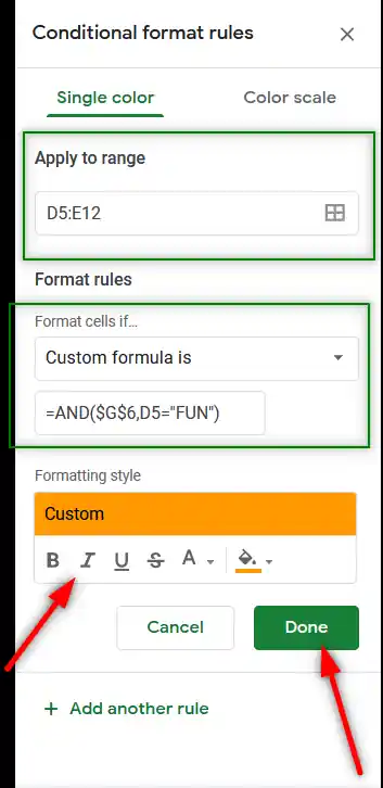
- We’ll apply this rule on the same data , so repeat all the steps.
- Enter the custom formula as =AND($G$6,D5=”FUN”).
- We chose the highlighted data to be in Yellow fill color this time.
The conditions applied will look like as shown in the picture below.
- After setting the required options, click DONE.
We are done and ready to use our checkboxes.
When using the example, if we check the box with HELLO CAPTION, all the HELLO words will be highlighted and so with the FUN CHECK BOX.
EXPLANATION OF THE FORMULA USED:
We have put multiple conditions over the same data which is evident from the process we just followed.
In the first section, we have used the custom formula as
The formula used is =AND($G$5,D5=”HELLO”).
Cell D5 contains the CheckBox.
We have put the two conditions in the AND FUNCTION which will return a TRUE only if both of the conditions are true, i.e. G5 i.e. the checkbox is selected, and D5=HELLO.
This function will be applied to all the range on which we applied the CONDITIONAL FORMATTING RULE.
Similarly the next function used is =AND($G$6,D5=”FUN”).
G6 contains the checkbox and D5 is the first cell which is equated to the FUN word. Both are passed as parameters in AND FUNCTION.
It’ll highlight the cell when both of the conditions are TRUE i.e. when the checkbox is selected and the text is FUN.
Let us try a few more examples.
EXAMPLE 2: HIGHLIGHT THE COMPLETE ROW BY CONDITIONAL FORMATTING USING CHECKBOX CONTROL
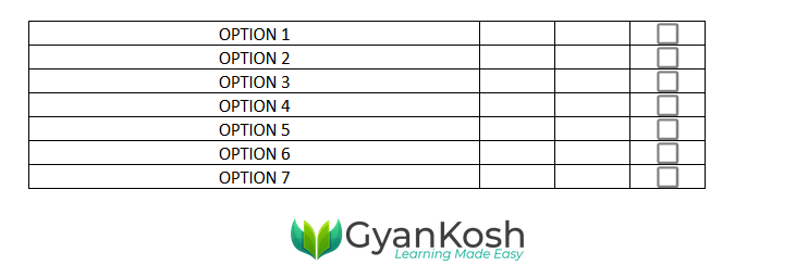
We can also control and highlight a complete row in the selected cell using conditional formatting and assigning this control to the checkbox.
FOLLOW THE STEPS TO HIGHLIGHT A ROW USING CONDITIONAL FORMATTING IN GOOGLE SHEETS:
- Select the data.
- Go to FORMAT menu and choose CONDITIONAL FORMATTING.
- The CONDITIONAL FORMATTING window will open on the right.
- APPLY TO RANGE shows the range on which we want to apply the conditional formatting. For our example, it’ll be B22:G28.
- As we selected the data before option, it’ll appear automatically.
- After setting the Range, choose CUSTOM FORMULA from the FORMAT RULES DROP DOWN .
- Enter the formula as =AND(B22:G22,J22).
- Set the format as per your requirement.
- Click DONE.
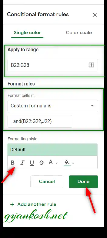
After we have clicked DONE, we are ready to go.
Let us try our example.
Simply check or uncheck the box. We can see that the options are selected as we select the corresponding checkbox.
EXAMPLE 3: HIGHLIGHT THE COMPLETE COLUMN BY CONDITIONAL FORMATTING USING CHECKBOX CONTROL
Just like the way we We can also control and highlight a complete row in the selected cell using conditional formatting and assigning this control to the checkbox.
FOLLOW THE STEPS TO HIGHLIGHT A COLUMN USING CONDITIONAL FORMATTING IN GOOGLE SHEETS:
- Select the data.
- Go to FORMAT menu and choose CONDITIONAL FORMATTING.
- The CONDITIONAL FORMATTING window will open on the right.
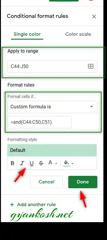
- APPLY TO RANGE shows the range on which we want to apply the conditional formatting. For our example, it’ll be C44:J50.
- As we selected the data before option, it’ll appear automatically.
- After setting the Range, choose CUSTOM FORMULA from the FORMAT RULES DROP DOWN .
- Enter the formula as =AND(C44:C50,C51).
- Set the format as per your requirement.
- Click DONE.
After we have completely put the setting into run, we can check the result.
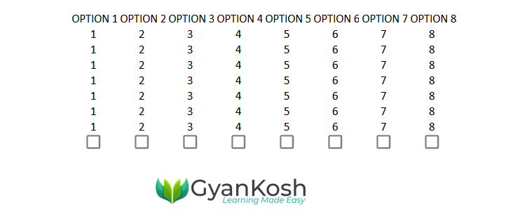
Following picture shows the running of this example.
After we have set the formulas, we can click the checkboxes to see if the column is being highlighted or not.
We can see in the picture below that our example works.
In this article we learnt the use of combining Conditional Formatting with the use of CHECK BOXES in Google Sheets.
FAQs
HOW TO CHANGE THE COLOR OF THE CHECKBOX IN GOOGLE SHEETS?
The CHECKBOX in Google Sheets behaves like a character only. You can change its color in very simple ways.
FOLLOW THE STEPS TO CHANGE THE COLOR OF THE CHECKBOX:
- Select the cell or cells containing the checkboxes.
- Go to FONT COLOR.
- Choose the FONT COLOR of your choice.
- The CHECKBOX COLOR will be changed.