Table of Contents
- INTRODUCTION
- WHAT IS CONDITIONAL FORMATTING BASED ON TEXT?
- HOW TEXT IS HANDLED IN GOOGLE SHEETS?
- WHAT IS CONDITIONAL FORMATTING BASED ON TEXT ?
- EXAMPLE 1: HIGHLIGHTING THE TEXT EQUAL TO SOME VALUE:
- RUNNING THE EXAMPLE
- EXAMPLE 2: HOW TO HIGHLIGHT THE TEXT WHICH MATCHES EXACTLY TO THE GIVEN TEXT ? [EXACT MATCH ]
- RUNNING THE EXAMPLE:
- EXAMPLE 3: HOW TO HIGHLIGHT THE CELLS IF TEXT CONTAIN A SPECIFIC CHARACTER
- RUNNING THE EXAMPLE
INTRODUCTION
Whenever we prepare any report in GOOGLE SHEETS, we have two constituents in any report.
The Text portion and the Numerical portion.
But just storing the text and numbers doesn’t make the super reports. Many times we need to automate the process in the reports to minimize the effort and improve the accuracy.
Many functions are provided by the GOOGLE SHEETS which work on Text and give us the useful output as well. But few problems are still left on which we need to apply some tricks with the available tools.
During the analysis , highlighting the values which fulfill any given condition is a very useful thing which can be done.
In this articles , we will continue learning many more techniques about the manipulation of text in GOOGLE SHEETS.
WHAT IS CONDITIONAL FORMATTING BASED ON TEXT?
CONDITIONAL FORMATTING is FORMATTING BASED ON THE CONDITIONS.
Formatting is the APPEARANCE BASED FEATURES such as font, fill color, font color , text size etc.
ANY CELL WHICH CONTAINS THE TEXT WHICH WILL FULFILL THE CONDITION WHICH WE SPECIFY, WILL BE HIGHLIGHTED WITH THE FORMAT WE HAVE CHOSEN.
It simply means that if we put the conditions on the Text, the list or table which is containing the different text values, will be highlighted.
For example, if we have long list and we want to search for some specific word, case specific search, any text containing any specific character or any other type of condition, we can make use of conditional formatting.
If you haven’t used this, kindly go through the link LEARN TO USE CONDITIONAL FORMATTING IN GOOGLE SHEETS for the introduction.
You’ll be amazed to see the capability of conditional formatting and its use which is awesome.
HOW TEXT IS HANDLED IN GOOGLE SHEETS?
TEXT is simply the group of characters and strings of characters which convey the information about the different data and numbers in GOOGLE SHEETS. Every character is connected with a code [ANSI].
Text comprises of the individual entity character which is the smallest bit which would be found in GOOGLE SHEETS.
We can perform the operations on the strings[Text] or the characters.Characters are not limited to A to Z or a to z but many symbols are also included in this which we would see in the later part of the article.
TEXT IS AN INACTIVE NUMBER TYPE[FORMAT] IN GOOGLE SHEETS. ANYTHING STORED AS TEXT [NUMBER OR DATE] WON’T RESPOND TO ANY STANDARD FORMULAS OR FUNCTIONS BUT SPECIALLY DESIGNED TEXT FUNCTIONS. [EXCEPTIONS DO OCCUR IN CASE OF NUMBERS]
If we need to make anything inactive, such as Date to be non responding to the calculation, we put it as a text. Similarly if we want to avoid any calculations for a number it needs to be put as a text.
WHAT IS CONDITIONAL FORMATTING BASED ON TEXT ?
CONDITIONAL FORMATTING is the process of formatting in GOOGLE SHEETS on the basis of the conditions. We can put many conditions in the cell and program the GOOGLE SHEETS to make the formatting , as desired, if the particular condition is met. Formatting comprises of the foreground color, background color, font, size etc. which are the properties of the text.
It makes the results more readable.
IT IS RECOMMENDED TO LEARN THE BASICS ABOUT CONDITIONAL FORMATTING, IF NOT VERY COMFORTABLE WITH THIS TOPIC.
CLICK HERE TO LEARN THE BASICS OF CONDITIONAL FORMATTING.
Maximum times, we apply the conditional formatting on the basis of values present in the cells.
Let us now learn the way by which we can apply the conditional formatting based on text.
EXAMPLES SHOWING CONDITIONAL FORMATTING BASED ON TEXT.
EXAMPLE 1: HIGHLIGHTING THE TEXT EQUAL TO SOME VALUE:
Let us find out the cell which contains a text value equal to some SPECIFIED TEXT.
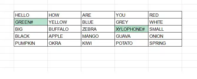
For the example let us take this block of text values in GOOGLE SHEETS.
| HELLO | HOW | ARE | YOU | RED |
| GREEN | YELLOW | BLUE | GREY | WHITE |
| BIG | BUFFALO | ZEBRA | XYLOPHONE | SMALL |
| BLACK | APPLE | MANGO | GUAVA | ONION |
| PUMPKIN | OKRA | KIWI | POTATO | SPRING |
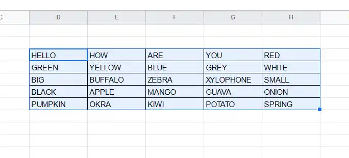
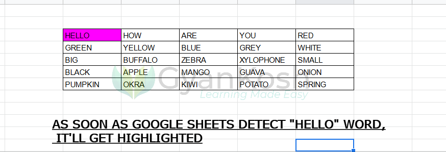
Let us try to highlight the cells containing HELLO.
It can be done in two ways.
1. Using the predefined options.
2. Using custom formula.
1. USING PREDEFINED OPTIONS
STEPS to highlight cells using the predefined option:
- Select the complete table.
- Go to FORMAT MENU >CONDITIONAL FORMATTING.
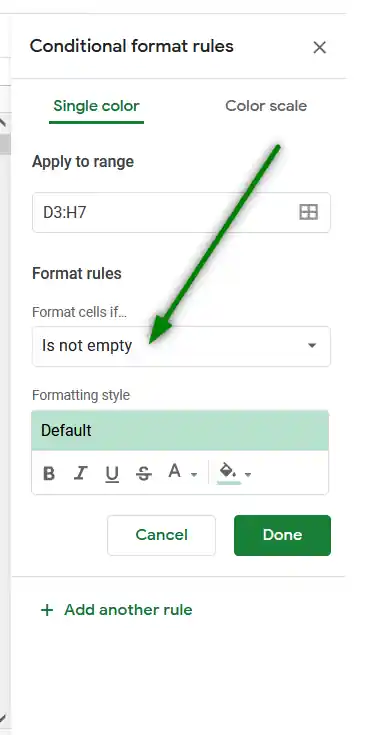
- The conditional formatting rules window will open on the right portion of the screen.
- In the rules, APPLY TO RANGE will be filled as we already selected the table before choosing the data otherwise put the range manually.
- Click FORMAT CELLS IF drop down to see more options.
- The location is shown in the picture below.
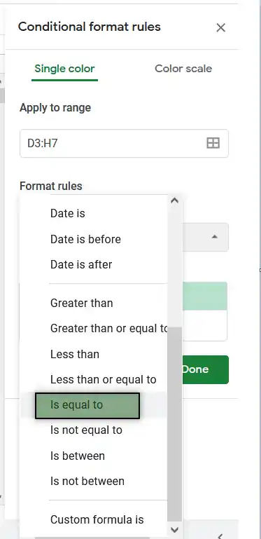
- Choose IS EQUAL TO from the drop down.
- Following dialog box will open.
- Enter the value in the field as shown in the picture.
- Select the format of the cells which satisfy the condition.
- and Click OK.
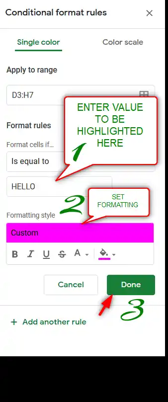
- As we click or choose IS EQUAL TO, some additional fields will open asking for the values.
- The following picture shows the screen.
- 1. Enter the value to be equated or highlighted.
- 2. Choose the formatting as per your requirement such as CELL FILL COLOR, bold , italic or underline, strikethrough or font color. This formatting will be given to the cells which contains the text fulfilling the given condition.
- 3. Click DONE.
- For our example, we want to highlight the word HELLO so we put HELLO word in IS EQUAL TO field.
- We chose the pink color as the cell fill color for the result.
- And clicked DONE.
All the cells containing HELLO word will be highlighted with a pink cell fill color.
NOTE: This method will HIGHLIGHT ALL THE TEXT INCLUDING hello, Hello, hellO or any other big small case combination which means there won't be any distinction on the basis of the case of the text.
2. USING CUSTOM FORMULA
We can get the same result by using the CUSTOM FORMULA too.
STEPS to highlight cells using the custom formula:
- Select the complete table.
- Go to FORMAT MENU>CONDITIONAL FORMATTING.
- The CONDITIONAL FORMATTING RULES window will open.
- Go to FORMAT CELLS IF drop down , scroll it down.
- Click the last option: CUSTOM FORMULA IS.
- A field will appear to enter the formula.
- Enter the formula in the field as =D3=”HELLO”. [D3 IS THE FIRST CELL OF OUR SELECTION. IF YOUR SELECTION’S FIRST CELL IS ANYTHING DIFFERENT, USE THAT ]
- Set the format as per your choice. We set the fill color as pink .[Don’t forget to change the format otherwise difference won’t be visible.]
- Click DONE.
- All the cells containing HELLO or hello will be highlighted.
Let us try our example.
RUNNING THE EXAMPLE
After putting all the conditions, let us try to see if it works or not.
In the following animated picture, we changed many cells to HELLO and you can see that the fill color changes as soon as the word is detected.
As we changed the text, the color is gone.
This method has an issue.
It’ll highlight the word HELLO and all the variants ignoring the case of the letters. It means it won’t give us an exact match for the conditional formatting in google sheets.
Let us try to remove this error and find out a method to exactly highlight the text.
EXAMPLE 2: HOW TO HIGHLIGHT THE TEXT WHICH MATCHES EXACTLY TO THE GIVEN TEXT ? [EXACT MATCH ]
In this example, let us find out the way to highlight the cells which contains the text same as some specified text exactly with the same content and with the same case.
In this example, we are taking a table of data for highlighting the text which satisfies the condition given.
We can also apply the same method to highlight the exact text using conditional formatting for the given List of the different data.
GENERALIZED FORMULA TO HIGHLIGHT THE EXACT TEXT:
=EXACT(FIRST CELL OF SELECTION, “TEXT TO BE MATCHED”).
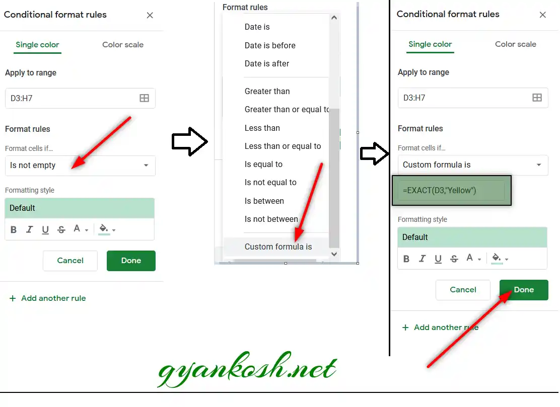
For our example, we will highlight the cell containing the text “Yellow”.
Follow the steps. [ THE FOLLOWING PICTURE CONTAINS THE STEPS IN THREE PORTIONS IN THE SAME PICTURE. LOOK AT IT FOR THE REFERENCE ].
- Select the complete table.
- Go to FORMAT MENU>CONDITIONAL FORMATTING.
- The CONDITIONAL FORMATTING RULES window will open.
- Go to FORMAT CELLS IF drop down , scroll it down.
- Click the last option: CUSTOM FORMULA IS.
- A field will appear to enter the formula.
- Enter the formula in the field as =EXACT(D3,”Yellow”). [D3 IS THE FIRST CELL OF OUR SELECTION. IF YOUR SELECTION’S FIRST CELL IS ANYTHING DIFFERENT, USE THAT ]
- Set the format as per your choice. We set the fill color as SEA GREEN .[Don’t forget to change the format otherwise difference won’t be visible.]
- Click DONE.
- All the cells containing HELLO or hello will be highlighted.
For the concept OF CONDITIONAL FORMATTING CLICK HERE.
RUNNING THE EXAMPLE:
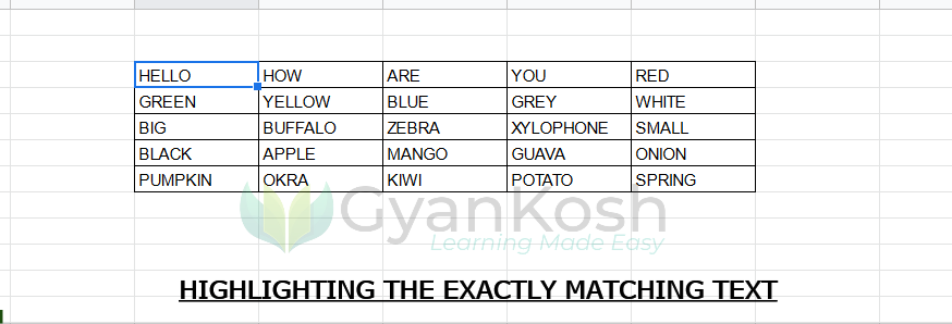
Let us try and check if the condition applied works or not.
We changed a few other cells with the different versions of the word YELLOW.
We can see that only the required text is highlighted.
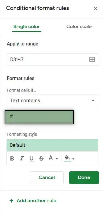
EXAMPLE 3: HOW TO HIGHLIGHT THE CELLS IF TEXT CONTAIN A SPECIFIC CHARACTER
Suppose we want to create a condition when we want to highlight the cell if the cell contains any specific character say # for our example.
GENERALIZED FORMULA TO HIGHLIGHT THE CELLS WHICH CONTAIN A SPECIFIC CHARACTER
- Select the complete table.
- Go to FORMAT MENU>CONDITIONAL FORMATTING.
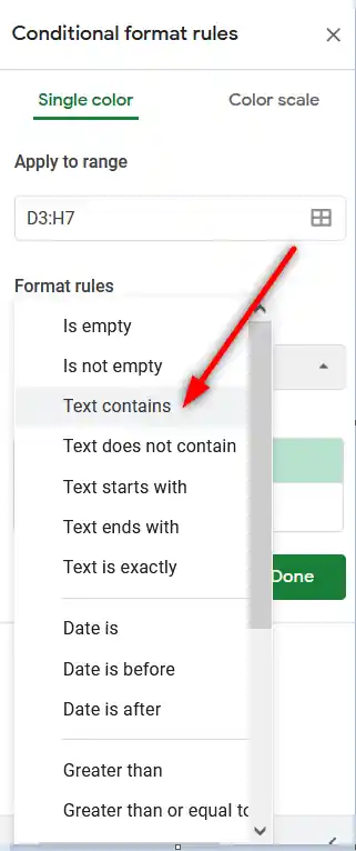
- The CONDITIONAL FORMAT RULES window will open.
- Choose TEXT CONTAINS from the FORMAT CELLS IF drop down.
- The field will appear.
- Enter the character or text portion in the field.
- For our example we’ll enter # in the field as shown in the picture below.
- Click DONE.
For the concept of CONDITIONAL FORMATTING CLICK HERE.
RUNNING THE EXAMPLE
After we have performed the steps, all the text containing the # will be highlighted as shown in the picture below.
These were a few examples of highlighting the text using conditional formatting in google sheets.
ONE MORE EXAMPLE FOR CONTROLLING THE CONDITIONAL FORMATTING WITH THE TEXT OR NUMBERS AT OTHER POSITION IS HERE.
CREATING A SIMPLE GANTT CHART IN GOOGLE SHEETS
LEARN USEFUL ARTICLES ABOUT GOOGLE SHEETS
THERE’S ALWAYS ROOM FOR IMPROVEMENT.
KINDLY GIVE YOUR VALUABLE SUGGESTIONS.