Table of Contents
- INTRODUCTION
- CREATING FIRST PIVOT TABLE USING VBA
- STANDARD STRUCTURE OF CREATING A PIVOT TABLE USING VBA
- CREATING CUSTOM CALCULATION IN PIVOT TABLE USING VBA
INTRODUCTION
PIVOT TABLES are one of the most powerful features of Excel.
Pivot Tables is a very old feature of the Excel which kept on getting better and better with the newer versions.
Pivot Tables help us to analyze large data within seconds as it requires no formulas, no dragging of functions, etc.
Just select the column of your needs, put them in the right section and the table is ready. There are many functions that can be directly applied in the PIVOT TABLE.
We have already learned to make use of PIVOT TABLES in the EXCEL BASICS.
If you want to revise kindly
CLICK HERE to learn how to use PIVOT TABLES IN EXCEL.
We’ll repeat the same process but now using VBA.
VBA will help us to automate our process and we can also take the help of pivot tables if needed. In this article, we’ll learn how to create pivot tables and manipulate them using VBA with the help of examples.
CREATING FIRST PIVOT TABLE USING VBA
Let us create our first PIVOT TABLE using VBA. We have the following data. States with a number of schools and colleges.
| COUNTRY | SCHOOLS | COLLEGES |
| UK | 19 | 66 |
| US | 17 | 37 |
| AUSTRALIA | 93 | 35 |
| FRANCE | 84 | 19 |
| SPAIN | 48 | 51 |
| UK | 12 | 64 |
| US | 22 | 24 |
| AUSTRALIA | 81 | 41 |
| UK | 62 | 89 |
| US | 77 | 80 |
| AUSTRALIA | 86 | 46 |
| FRANCE | 55 | 94 |
| UK | 64 | 97 |
| US | 71 | 54 |
| AUSTRALIA | 45 | 40 |
| FRANCE | 81 | 98 |
| UK | 66 | 17 |
| US | 95 | 83 |
| AUSTRALIA | 32 | 90 |
| FRANCE | 73 | 27 |
| SPAIN | 41 | 23 |
We can observe that there are many entries for a particular category.
For example, many countries have so many entries.
OBJECTIVE
CREATE A PIVOT TABLE USING THE GIVEN DATA
Make use of VBA to enter the given text into cell positioned at location D3.
PLANNING THE SOLUTION
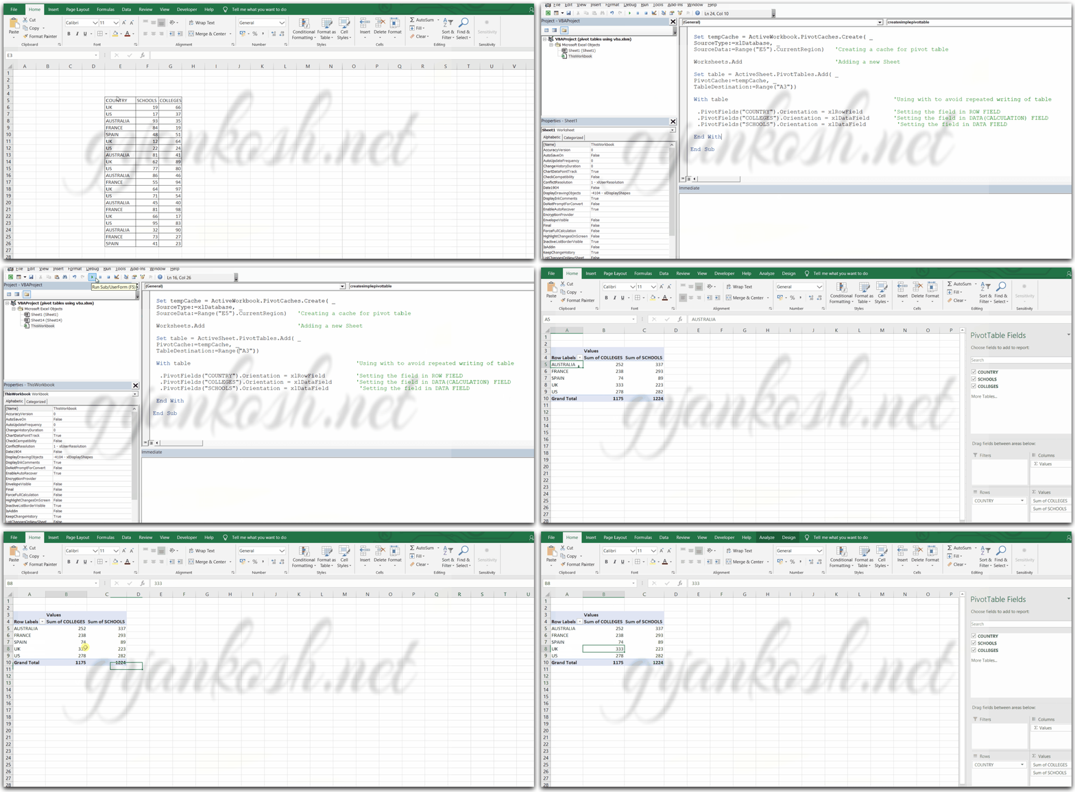
We’ll use the standard procedure to create a PIVOT TABLE. After creating we’ll put COUNTRY in the ROW FIELDS and SCHOOLS AND COLLEGES in the DATAFIELDS.
CODE
'gyankosh.net
'creating a pivot table using VBA

Sub createsimplepivottable()

Dim tempCache As PivotCache

Dim table As PivotTable

Set tempCache = ActiveWorkbook.PivotCaches.Create( _
SourceType:=xlDatabase, _
SourceData:=Range("E5").CurrentRegion) 'Creating a cache for pivot table

Worksheets.Add 'Adding a new Sheet

Set table = ActiveSheet.PivotTables.Add( _
PivotCache:=tempCache, _
TableDestination:=Range("A3"))

With table 'Using with to avoid repeated writing of table

.PivotFields("COUNTRY").Orientation = xlRowField 'Setting the field in ROW FIELD

.PivotFields("COLLEGES").Orientation = xlDataField 'Setting the field in DATA(CALCULATION) FIELD

.PivotFields("SCHOOLS").Orientation = xlDataField 'Setting the field in DATA FIELD

End With

End Sub
EXPLANATION
We declare tempCache as PivotCache which is needed for the PIVOT TABLE CREATION and a pivot table variable as temptable.
After this we pick the range from the sheet using the statement
Set tempCache = ActiveWorkbook.PivotCaches.Create( _
SourceType:=xlDatabase, _
SourceData:=Range(“E5”).CurrentRegion)
Source data is the region starting from cell E5.
It means our data is present in E5.
The current region will consider all the contiguous data. The data which is connected with adjacent cells.
After this, we add a new sheet.
There we take out the PIVOT TABLE and settable from the cache mentioning the cell as A3 i.e. the table should start from A3.
After the table is ready, we’ll set the fields to the data which we put in pivot tables.
We put the country in the row field and the rest in the data fields.
The output is shown below.
RUNNING THE CODE AND OUTPUT
STANDARD STRUCTURE OF CREATING A PIVOT TABLE USING VBA
BEFORE MOVING ON TO THE NEXT EXAMPLE, LET US UNDERSTAND THE BASIC STRUCTURE OF CREATING A PIVOT TABLE.
If we notice the last example, we can have a rough idea about the structure of the PIVOT TABLE in VBA.
Let us remember this structure so that we can finalize this.
Have a look at the structure below. This is the standard structure of the pivot table.
STRUCTURE OF THE PIVOT TABLE
STANDARD STEPS FOR A PIVOT TABLE CREATION
SUB PROCEDURE NAME
‘These two variables will be there always. Name can be as per your choice.
Dim tempCache As PivotCache
Dim table As PivotTable
Setting the table range to the Cache by passing the range.
Set tempCache = ActiveWorkbook.PivotCaches.Create( _
SourceType:=xlDatabase, _
SourceData:=Range(“E5”).CurrentRegion)
‘Setting the pivot table at destination given by range.
Set table = ActiveSheet.PivotTables.Add( _
PivotCache:=tempCache, _
TableDestination:=Range(“A3”))
Setting up the the required fields
.PivotFields(“COUNTRY”).Orientation = xlRowField ‘Setting the field in ROW FIELD
End Sub
CREATING CUSTOM CALCULATION IN PIVOT TABLE USING VBA
OBJECTIVE
CREATING A PIVOT TABLE WITH A CUSTOM CALCULATION
DATA
We have data about the daily rain in centimeters of a city. The data is random containing the details such as the rainfall and month. We need to find the average rainfall in the city per month.
The data is following.
| RAINFALL IN CITY A | |
| MONTH | RAINFALL |
| APRIL | 5.6 |
| MAY | 5.7 |
| JUNE | 6.8 |
| JULY | 9.6 |
| AUGUST | 9.7 |
| SEPTEMBER | 9.8 |
| OCTOBER | 8.1 |
| NOVEMBER | 5.4 |
| DECEMBER | 8.7 |
| OCTOBER | 8.2 |
| NOVEMBER | 7.3 |
| DECEMBER | 9.1 |
| JANUARY | 5.8 |
| JANUARY | 6.9 |
| FEBRUARY | 5 |
| NOVEMBER | 6.8 |
| DECEMBER | 9.9 |
| OCTOBER | 7.1 |
| NOVEMBER | 10 |
| DECEMBER | 7.4 |
| OCTOBER | 6.4 |
| NOVEMBER | 5.8 |
| DECEMBER | 5.3 |
CODE
'gyankosh.net
'FINDING OUT AVERAGE RAINFALL PER MONTH USING PIVOT TABLES IN VBA

Sub averageRainfall()

Dim tempCache As PivotCache

Dim table As PivotTable

Set tempCache = ActiveWorkbook.PivotCaches.Create( _
SourceType:=xlDatabase, _
SourceData:=Range("F5", "G28")) 'Creating a cache for pivot table

Worksheets.Add 'Adding a new Sheet
Set table = ActiveSheet.PivotTables.Add(PivotCache:= _
tempCache, TableDestination:=Range("f5"))
MsgBox ("I M AT 1")


With table 'Using WITH to avoid repeated writing of table
.PivotFields("MONTH").Orientation = xlRowField

.CalculatedFields.Add "remarks", "=RAINFALL"

.PivotFields("remarks").Orientation = xlDataField

.PivotFields("sum of remarks").Caption = "TOTAL RAINFALL"

.PivotFields("RAINFALL").Orientation = xlDataField

.PivotFields("sum of RAINFALL").Function = xlAverage

.PivotFields("average OF RAINFALL").Caption = "AVERAGE"

End With

End Sub
EXPLANATION
Let us check the explanation of introducing a custom field in the pivot table using VBA.
We start with a declaration of PIVOT CACHE and PIVOT TABLE.
We pass the values to the PIVOT CACHE with a range declared by F5:G28 which is the range of the data.
We add a new sheet.
We pass the output range to the PIVOT TABLE and create it from the CACHE.
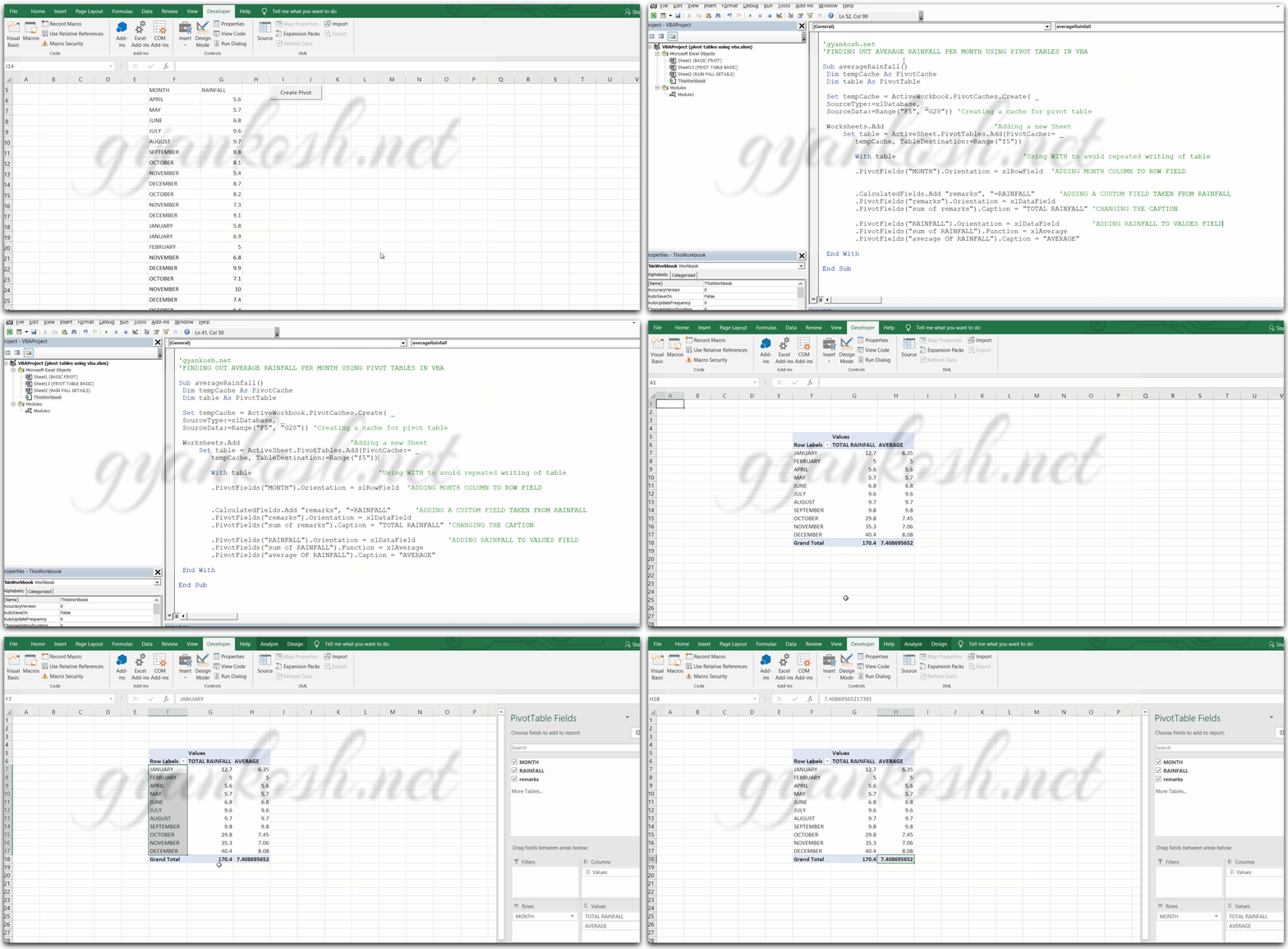
The output range is set as F5. But this F5 will be of the new sheet which we just created. Now the table is created and we need to fix its fields into different options like row or column of data. We put the MONTHS in a row field. We add a temporary custom field named remarks in which we pass the values of RAINFALL.
We put this as a data field that gives us the monthly sum of the rainfall.
NOTICE THE NAMES USED.
Pivot table immediately changes the name and we need to refer to those fields with the changed name.
We again change the caption to the one we need. After this, we again put the field RAINFALL and change its function to average.
We again change its caption. The following picture shows the running process.
THE CUSTOM FIELD IS USED AS FOLLOWS:
table.calculatedfields.Add “name of the field” “formula”
Formula can be anything connected with the field names.

