Table of Contents
INTRODUCTION
If you have been using the MICROSOFT EXCEL software for some time, you must have heard or read about the word POWER QUERY.
POWER QUERY IS A DATA SHAPING TOOL WHERE WE CAN BRING THE DATA THROUGH A CONNECTION FROM VARIOUS SOURCES, DO SOME SHAPING SUCH AS REMOVING ROWS, COLUMNS, CHANGING DATA TYPES, TRIMMING THE DATA ETC. AND GET IT READY , FINALLY FOR THE ANALYSIS IN OUR MAIN SOFTWARE SUCH AS MICROSOFT EXCEL OR MICROSOFT POWER BI .
FOR THE INTRODUCTION OF POWER QUERY, CLICK HERE.
Power Query tool, in fact, has immense powers to shape up the data in the way we want.
We’ll cover a lot of practical problems to sort them out with the help of the POWER QUERY.
IN THIS ARTICLE, WE ‘LL LEARN TO CONCATENATE COLUMN DATA INTO A NEW COLUMN
WHAT IS CONCATENATION
CONCATENATION or TO CONCATENATE simply means the process of sticking together.We use this process with the use of function or operator in Excel to stick any two or more texts, numbers or numbers and texts.For example
1 concatenated with 2 will result in 12.
Hello concatenated with Sir will result in HelloSir.
[ We didn’t put any spaces in between. If we put a space after Hello or before Sir, the result will be Hello Sir.]
HOW TO CONCATENATE COLUMNS IN POWER QUERY
We will take an example to understand the process of concatenating the columns to create a new column.
Let us take a table for the example which we will load from the EXCEL and transform it so that its loaded into POWER QUERY EDITOR.
CLICK HERE TO LEARN HOW TO GET DATA FROM EXCEL INTO POWER BI
The table for the example is shown in the picture below.
Read the article mentioned above.
In the navigator, use TRANSFORM DATA and the table would open in the POWER QUERY EDITOR.
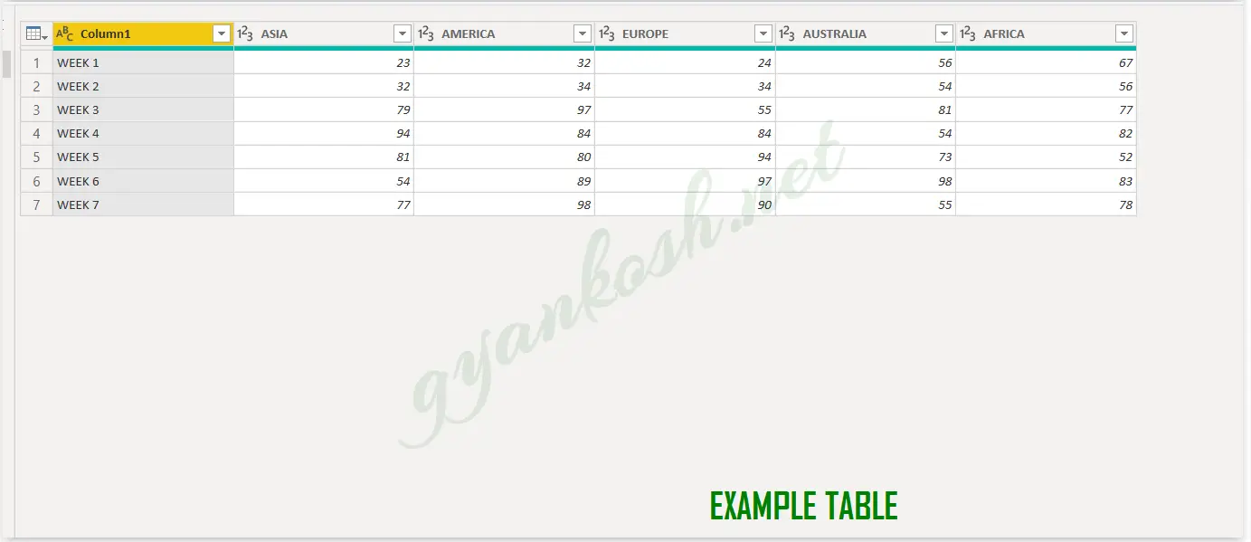
DATA FOR THE EXAMPLE
FOLLOWING PICTURE SHOWS THE DATA FOR THE EXAMPLE.
We have the sales data for 7 week from the different continents.
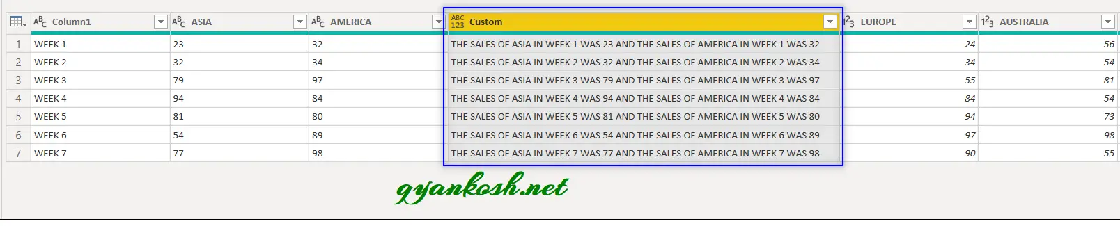
We will create a new column containing the Text The sales of ASIA in WEEK 1 was ….. and the sales of AMERICA in Week 1 was …..
For this, we’ll be requiring three columns i.e. COLUMN 1, COLUMN ASIA, COLUMN AMERICA.
Let us see how we can achieve this.
PREREQUISITES FOR CONCATENATION:
If you already tried to concatenate the columns in the EXCEL STYLE, you might have ended up with an error in the values. That is because of the reason that we can’t concatenate just any format but only TEXT FORMAT.
All the columns being concatenated should be in the TEXT FORMAT.
For our example, COLUMN 1 is already text but COLUMN ASIA and COLUMN AMERICA are in the number format.
So we need to convert the format to the text format first.
FOLLOW THE STEPS TO CHANGE THE FORMAT OF THE COLUMN IN POWER QUERY.
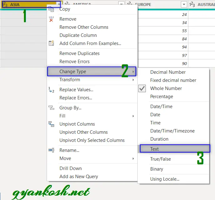
- Right click the column header ASIA.
- The following menu will appear.
- Go to CHANGE TYPE and choose TEXT.
- Repeat the process for COLUMN AMERICA also.
STEPS TO CONCATENATE COLUMNS IN POWER QUERY AND CREATE A NEW COLUMN:
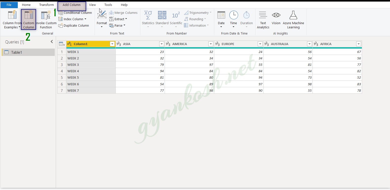
- Select TAB ADD COLUMN.
- Click on CUSTOM COLUMN button.
- The location is shown in the picture below.
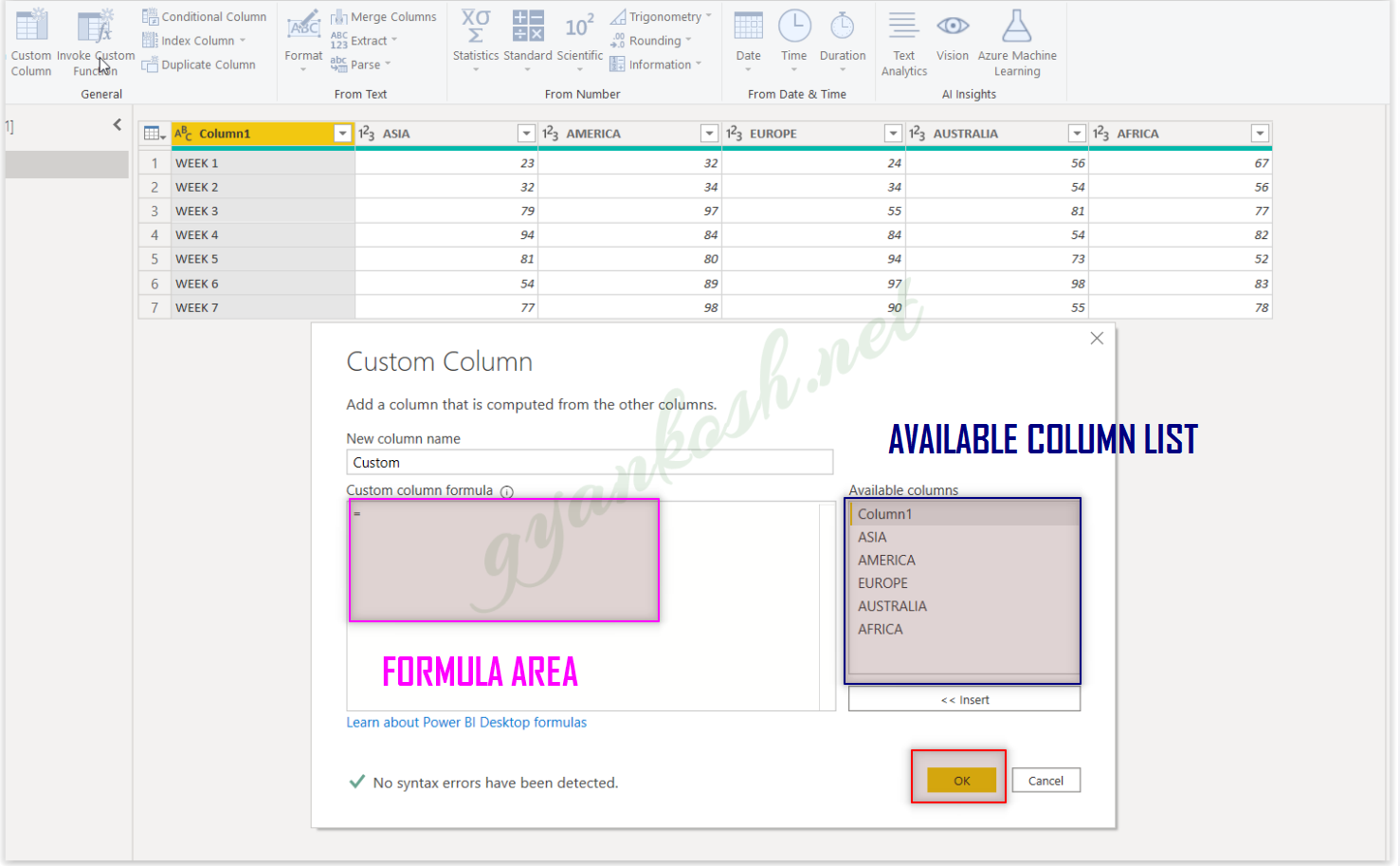
After clicking the CUSTOM COLUMN button, CUSTOM COLUMN DIALOG BOX will open.
The picture below shows the CUSTOM COLUMN DIALOG BOX.
The dialog box asks for the COLUMN NAME, Asks for the FORMULA [ which will derive the values in the new column ] and provides the available column names of the current table.
THE NOTIFICATION IN THE LOWER PORTION OF THE CUSTOM COLUMN DIALOG BOX SHOWS THE STATUS OF THE SYNTAX ERROR.
For our example we put the NEW COLUMN NAME as CUSTOM.
Put the formula for the concatenation as =”THE SALES OF ASIA IN “&[Column1]&” WAS “&[ASIA]&” AND THE SALES OF AMERICA IN “&[Column1]&” WAS “&[AMERICA]
We don’t need to write the column names. Choose the column names from the available list on the right, select it and click INSERT button at the bottom. The name will appear in the FORMULA AREA.
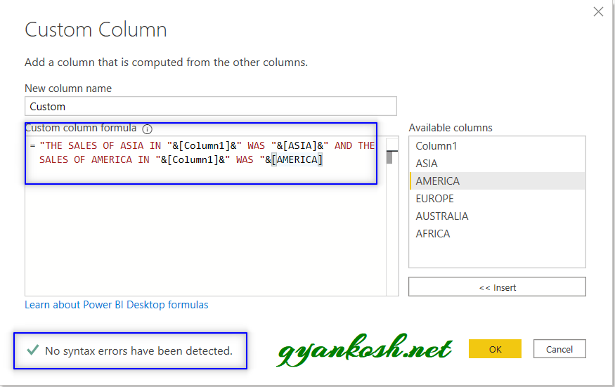
- Check the syntax notification at the bottom. If it says NO ERROR as in our case, click OK.
- The new CUSTOM COLUMN will be added on the RIGHT of the table. The location can be easily changed by RIGHT CLICK>MOVE>LEFT, RIGHT, TO THE END OR TO THE BEGINNING.