PROVIDING ACCURATE, RELIABLE AND STRAIGHT TO THE POINT KNOWLEDGE ABOUT DIFFERENT IT TOOLS EXPLAINED WITH PRACTICAL EXAMPLES

WHAT IS POWER QUERY? HOW TO USE POWER QUERY?

INTRODUCTION

If you have been using the MICROSOFT EXCEL software for some time, you must have heard or read about the word POWER QUERY.

POWER QUERY IS A DATA SHAPING TOOL WHERE WE CAN BRING THE DATA THROUGH A CONNECTION FROM VARIOUS SOURCES, DO SOME SHAPING SUCH AS REMOVING ROWS, COLUMNS, CHANGING DATA TYPES, TRIMMING THE DATA ETC. AND GET IT FINALLY FOR THE ANALYSIS IN OUR MAIN SOFTWARE SUCH AS MICROSOFT EXCEL OR MICROSOFT POWER BI .

This is an amazing tool in fact which has additional tools which are not available in the STANDARD EXCEL [ Although it is a part of the EXCEL only ]. Once the user starts using it, only then he would be able to feel the ease by which it handles the data and does some of the magnificent jobs.

The main steps of using the POWER QUERY are:

Connecting the source.
Transforming the data.
Getting it to the main software.
Create charts, reports or dashboards. [Job done in the main application ]

In this article, we would learn the basics of the POWER QUERY. The article is meant for the learners who are the first time users of POWER QUERY.

HOW TO OPEN POWER QUERY EDITOR IN EXCEL

POWER QUERY has a separate environment which opens up as a separate entity.

We have power query in EXCEL as well as in POWER BI. Let us find out the process of opening the POWER QUERY in both.

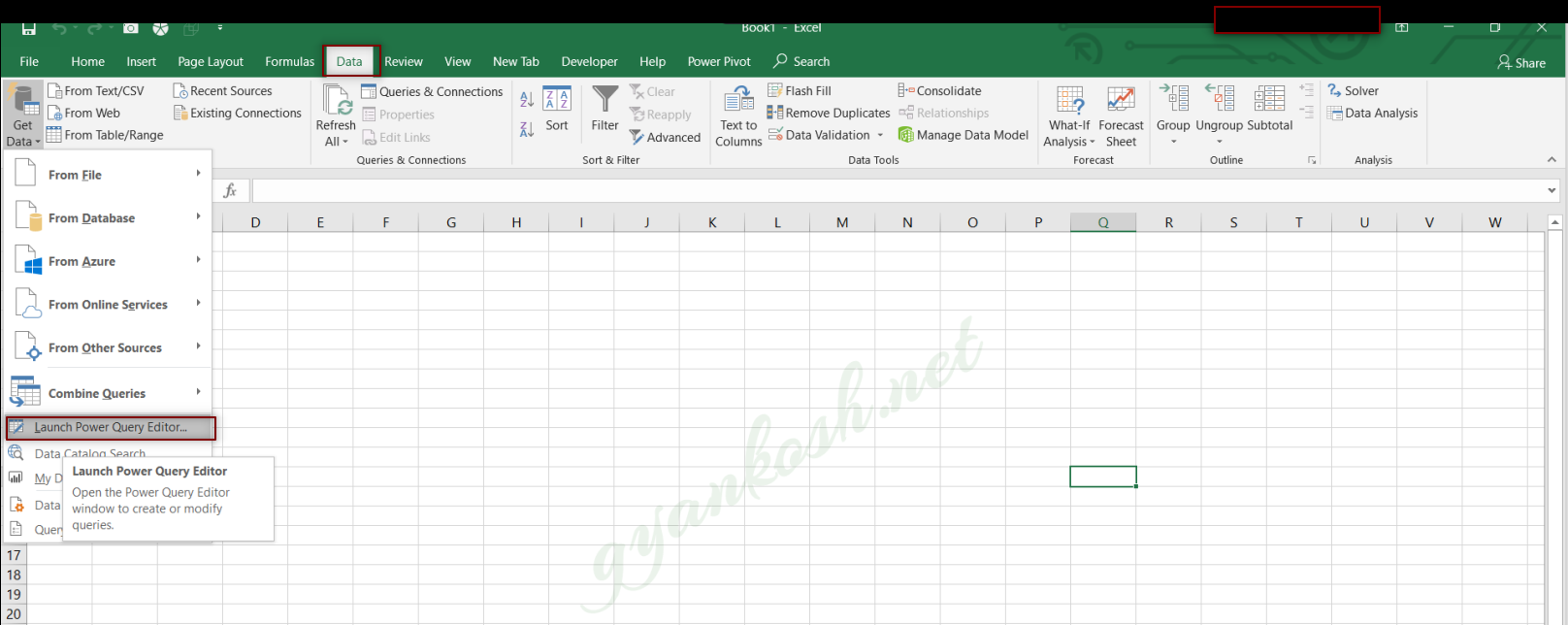
STEPS TO OPEN POWER QUERY IN EXCEL 2019.

Go to DATA TAB>GET DATA> LAUNCH POWER QUERY

FOR OTHER VERSIONS CLICK HERE.

INTRODUCTION TO THE VARIOUS PARTS OF THE POWER QUERY

Let us get acquainted with the working environment of POWER QUERY.

LET US UNDERSTAND THE VARIOUS AREAS OF THE POWER QUERY EDITOR.

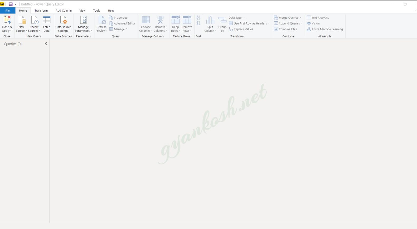
LOOK AT THE PICTURES BELOW. The two pictures refer to the POWER QUERY available in the MICROSOFT EXCEL and POWER BI.

Both are almost same with a few changes in the placement of the options. The pictures below can be looked at for the difference.

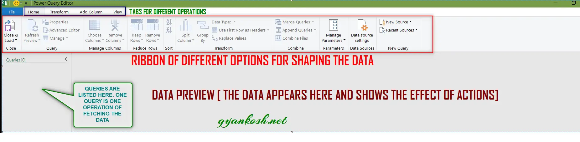
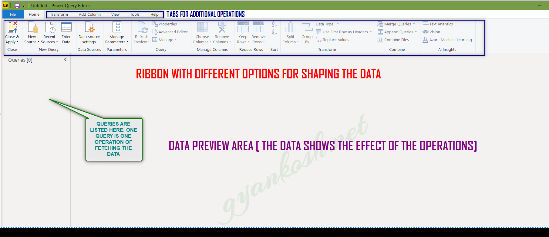
1.RIBBON:

The upper portion of the editor contains the RIBBON with different tabs. The ribbon contains the ready to use functionalities of the POWER QUERY EDITOR. We’ll learn all the functionalities in the next articles.

2.DATA PREVIEW:

It is the area where our data is visible. We apply the operations on the data such as column removal, data type change etc. , all are previewed here before finalizing.

3.NAVIGATOR PANE / QUERIES LIST [ON THE LEFT PART OF THE EDITOR] :

It shows the list of all the queries.

ONE QUERY WOULD MEAN TO FETCH DATA FROM A SOURCE.

It’ll be shown in this list. Suppose we fetched data from the EXCEL in one query, then from the web, then from the csv etc. , so it means we’ll have three queries which will be listed in the NAVIGATOR PANE.

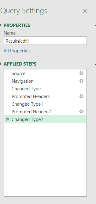
4.QUERY SETTINGS PANEL:

This panel is not visible in the pictures below. It comes when we start editing the query.

It records all the steps taken by us and gives us an easy access to revert back to any step directly.

For example, suppose we renamed a column and deleted other. Both of these steps will be recorded and shown in the QUERY SETTING PANEL.

POWER QUERY EDITOR NEVER ALTERS THE ORIGINAL DATA BUT JUST BRING THE DATA AND THEN TRANSFORMS IT AS PER NEED.

CREATING POWER QUERY : EXAMPLE

Before we move further, let us take a simple example and shape it using POWER QUERY to understand the basic working of POWER QUERY.

Here is the list of steps.

Launching the POWER QUERY EDITOR.
Fetching the data into power query.
Shaping it.
Sending it to the main application for further processing.

Bring a table from the web for the world cup cricket results 2019, clean the data and put it in excel.

https://en.wikipedia.org/wiki/Cricket_World_Cup

LAUNCHING THE POWER QUERY EDITOR

The first and foremost steps is to launch the query editor.

The procedure has already been discussed.

Go to DATA TAB> GET DATA> LAUNCH POWER QUERY EDITOR.

The editor will open.

FETCHING THE DATA FROM THE SOURCE

POWER QUERY is really flexible when it comes to the choices from where we can get the data from.

We’ll cover all the main sources but for this example, as given in the problem, we have been provided with a link from where we need to get the RESULT TABLE.

The link as already mentioned is https://en.wikipedia.org/wiki/Cricket_World_Cup.

Let us get the data from this link.

STEPS TO FETCH THE DATA FROM WEB TO THE POWER QUERY:

Go to HOME TAB>NEW SOURCE> OTHERS>WEB.
The location is shown in the picture below.

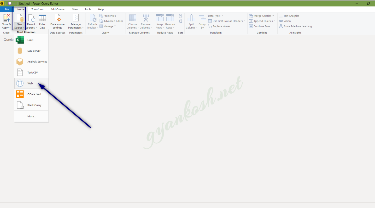
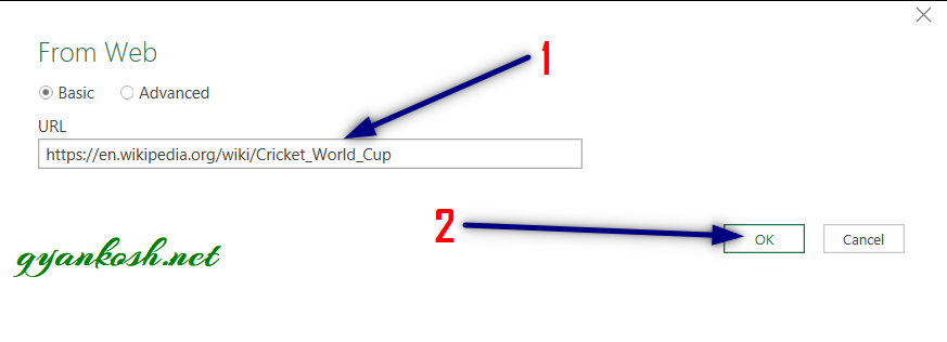
After we click WEB, a small window will open asking for the link.

Put the given link https://en.wikipedia.org/wiki/Cricket_World_Cup in the field as shown in the picture below and click OK.

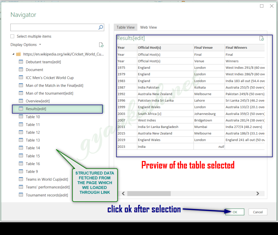
POWER QUERY would load the page and filter out the structured data from the page like tables and enlist them in the navigator as shown in the picture below.

NAVIGATOR SHOWS THE COMPLETE DATA FETCHED FROM THE SOURCE. IT LETS US CHOOSE THE RELEVANT DATA OF OUR USE AND DISCARDS THE REST.

Choose the relevant table from the list of the data got from the link.
Select the table.
Check the preview on the right side previewing pane.
Click OK.
The data will be loaded in the POWER QUERY EDITOR.

After we click WEB, a small window will open asking for the link.

Put the given link https://en.wikipedia.org/wiki/Cricket_World_Cup [copy it from here] in the field as shown in the picture below and click OK.

POWER QUERY would load the page and filter out the structured data from the page like tables and enlist them in the navigator as shown in the picture below.

NAVIGATOR SHOWS THE COMPLETE DATA FETCHED FROM THE SOURCE. IT LETS US CHOOSE THE RELEVANT DATA OF OUR USE AND DISCARDS THE REST.

Choose the relevant table from the list of the data got from the link.
Select the table.
Check the preview on the right side previewing pane.
Click OK.
The data will be loaded in the POWER QUERY EDITOR.

By this step, the data has been fetched into the POWER QUERY EDITOR.

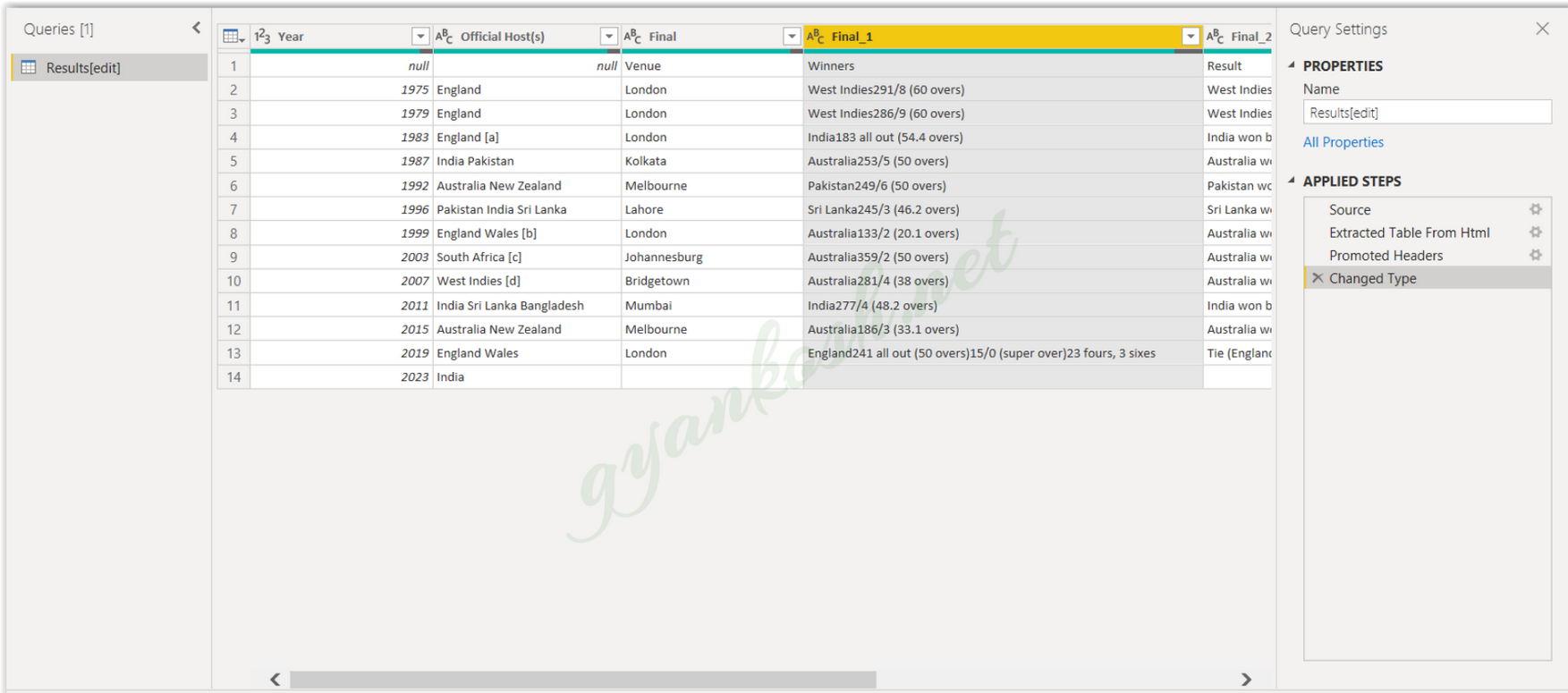
SHAPING THE DATA

Now, we come to the main task of the power query editor. Here are our objective list:

Only first four columns are needed.
The fourth column should have only the winning team name.
The column names should be YEAR, OFFICIAL HOST, VENUE AND WINNERS.
For these three objective, we’ll transform the data one by one.

STEPS TO REMOVE COLUMNS IN POWER QUERY EDITOR:

We have two options available for this process.

We can select the columns to be RETAINED and remove the other columns or
We can select the columns to be REMOVED and keep the columns which are to be kept.

FOR REMOVING THE COLUMNS WHICH ARE NOT SELECTED:

Select the column by clicking on its header.[ For multiple selection keep the CTRL BUTTON pressed till the right click operation is done]
Right click and choose REMOVE OTHER COLUMNS, if we have selected the columns which we want to retain.

*This option is shown in the process below in the animated picture.

FOR REMOVING THE COLUMNS WHICH ARE SELECTED:

Select the columns by clicking on the headers. [ For multiple selection keep the CTRL BUTTON pressed till the right click operation is done]
Right Click on the selected portion and select REMOVE THE COLUMNS.
The selected columns will be removed from the table.

REMOVING THE NUMBERS FROM THE FOURTH COLUMN

Our aim is not only to remove the numbers but to remove everything after the country name.

A ready option is available for this task in the POWER QUERY.

STEPS TO REMOVE THE CONTENT AFTER THE COUNTRY NAME:

Select the column number 4 which contains the winning team name and RIGHT CLICK.
Choose SPLIT COLUMN> BY NON DIGIT TO DIGIT.
This option would start from the left and split the columns in to many columns with the condition that the column would start from non digit to digit. We need only the first column which would start from the letters and end at the character where number starts.
Delete all the other columns by selecting them and pressing right click>remove columns

The process is given in the following animated picture.

RENAMING THE COLUMN HEADERS AND REMOVING NULL ROWS

Now , the last steps is to rename the COLUMN HEADERS and remove the row with the null values.

STEPS TO RENAME THE COLUMN HEADERS.

DOUBLE CLICK the column header.
The name would become editable.
Put the name of your choice. For our example, we would give the names as YEAR, OFFICIAL HOST, VENUE AND WINNER.
The next step is to remove the first line containing the NULL values.
Open the drop down in the header of the first column [YEAR COLUMN] and deselect null. This step would remove the complete row containing the row null.

*The complete process is shown in the animated picture below.

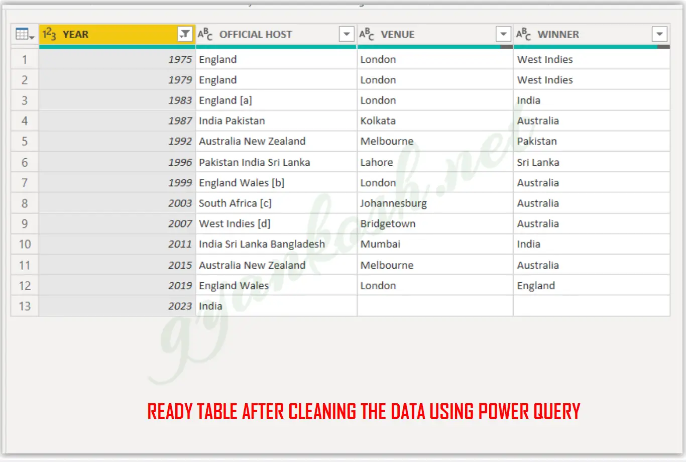
We have completed all the objectives and our data is clean and ready for the analysis now.

We can click CLOSE & APPLY which is the first button in the first data tab of ribbon. query will be closed and the ready data will be transferred to the application whether it is EXCEL or POWER BI.

The following picture shows the clean data which is ready.

Contents