Table of Contents
- INTRODUCTION
- WHAT IS ADVANCED FILTER IN EXCEL?
- EXAMPLE: USE ADVANCED FILTER TO FILTER THE GIVEN DATA
- HOW TO ENTER CRITERIA IN ADVANCED FILTER IN EXCEL?
- HOW TO ENTER FORMULA
- HOW TO ENTER MULTIPLE CONDITIONS IN ADVANCED FILTER IN EXCEL?
- MULTIPLE CONDITION
- FAQs
- HOW EXCEL FILTER REMOVES THE UNWANTED DATA?
- WHY THE RESULT DIDN’T UPDATE WHEN I CHANGED THE CONDITIONS IN ADVANCED FILTER IN EXCEL?
- HOW TO CLEAR OR REMOVE ADVANCED FILTER IN EXCEL?
- WHAT IS THE KEYBOARD SHORTCUT TO APPLY ADVANCED FILTER?
INTRODUCTION
In practical applications, in maximum cases, we have a large data that can’t be managed by just having a look at the data and manually selecting it.
If we want to search for a particular data, we can do that by using control + F and then typing but it is again a cumbersome task to use it over and again and type the search word.
For these reasons, we have got an option called FILTER which we discussed in another post.
But FILTER deals with simple properties and predefined formulas. What if the condition which we want is not present in the predefined conditions.
For such cases, there is an additional option known as the ADVANCED FILTER in EXCEL.
Advanced filters are used for a more complex filtering process. It is done in a different style.
Let’s try to understand it with the help of an example.
ADVANCED FILTER gives a dialog box to be filled as per the need of the criteria.
In this article, we’d learn about the need for advanced filters and learn how to use the advanced filter to filter data for more complex situations.
WHAT IS ADVANCED FILTER IN EXCEL?
Filters are used to remove the things which are not required. For example, if we use the filter on water, the impurities will be removed from the water.
Similarly, we have FILTERS in EXCEL which are very helpful to filter out the data which is important to us and hide the data which is not useful while analyzing the data.
We already learned FILTERS here. But what if we want to filter the data on more complex conditions.
Well, in that case, we have the option of ADVANCED FILTERS.
ADVANCE FILTERS lets us apply the custom formulas that will be used to filter our data.
EXAMPLE: USE ADVANCED FILTER TO FILTER THE GIVEN DATA
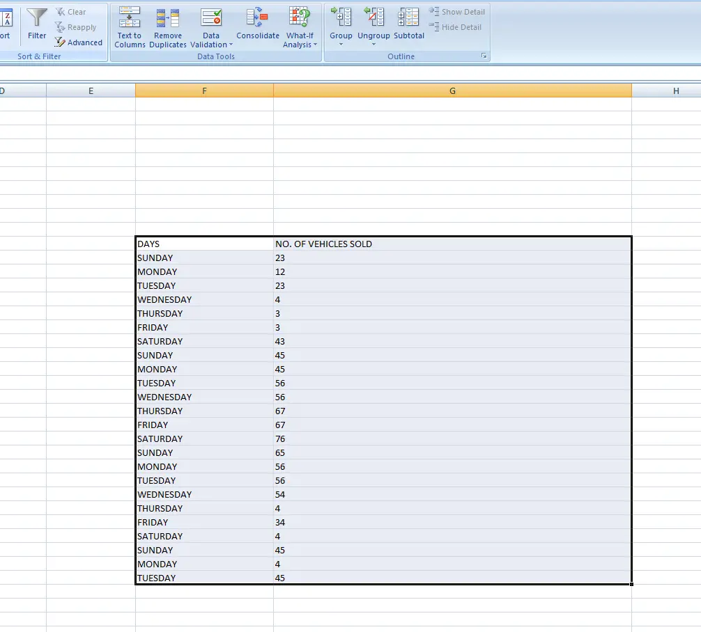
The example shows the weekdays with the number of vehicles sold for a few weeks.
Let us use an advanced filter to find out the different data.
FOLLOW THE STEPS TO APPLY ADVANCED FILTER IN EXCEL:
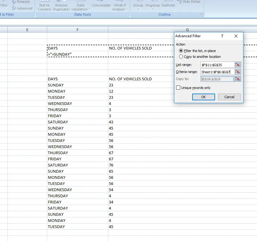
- Select the whole data sample and click Advanced Filter.
- After clicking the ADVANCED button, a dialog box will open.
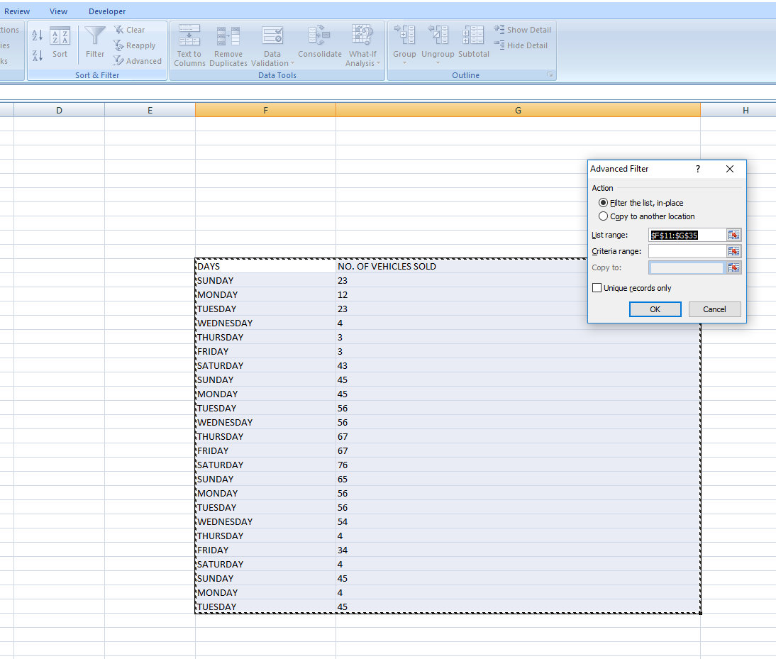
- The LIST RANGE should be the first cell up to the last cell of the data including the column HEADINGS. It is the data on which the filter will be applied.
- If we click ok, nothing will happen at this stage. If we put a new STARTING CELL in COPY TO, it’ll copy the complete data to that particular location.
*Kindly select the radio button "Copy to another location" for this feature otherwise the field will be disabled.
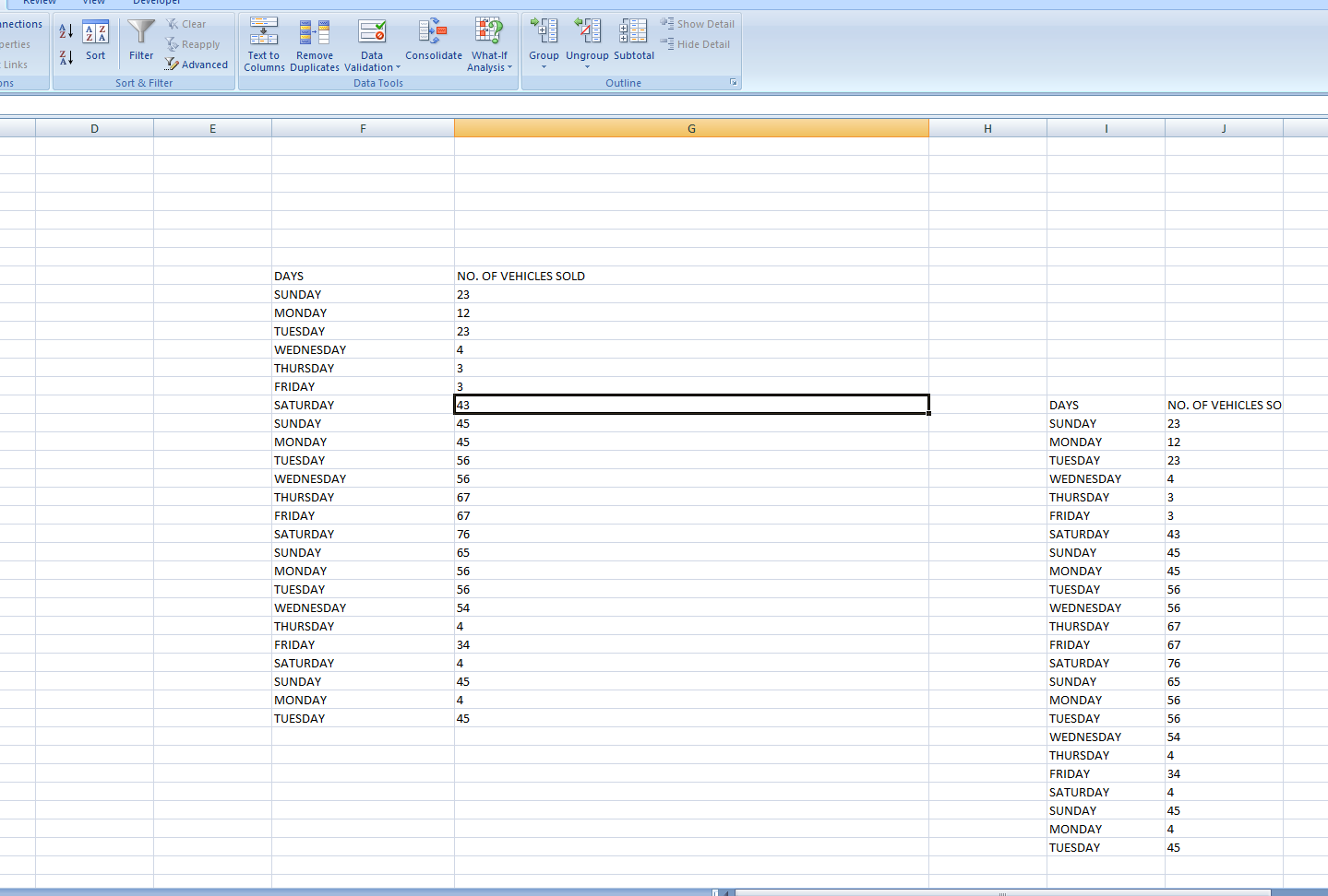
Enter the address in the cell where you want to copy the data.
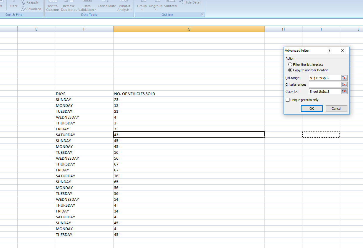
- If you want to copy the data. Enter the starting cell.
HOW TO ENTER CRITERIA IN ADVANCED FILTER IN EXCEL?
CRITERIA in the advanced option is written in an almost similar fashion to the table.
CREATE A TABLE OF THE CRITERIA WITH THE HEADINGS SAME AS THAT OF THE DATA.
FOLLOW THE STEPS TO ENTER THE CRITERIA:
- Select a different area for the criteria.
- Put the heading of the table (data on which the filter is to be applied) on the top. In this example,we have put Days and number of vehicle sold as headings same as the original data sample.
- Enter the condition.
- Enter the list of the cell containing the condition in the Dialog box in CRITERIA field.
HOW TO ENTER FORMULA
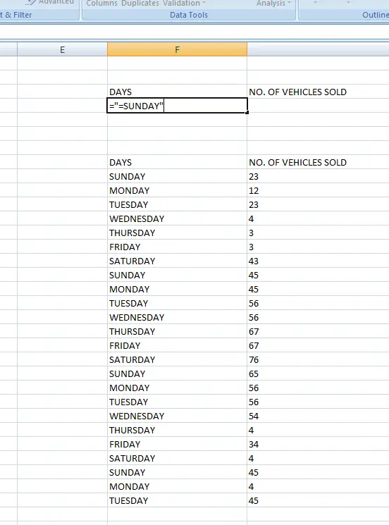
The formula is put in the condition cells as the following format
=”condition”
e.g. =”=SUNDAY” means to equate the days to SUNDAY.
The first “=” will go away as you press Enter. If you want to show it you can do this by clicking CTRL+`. Although there won’t be any difference in the result.
A few more formula options are <,>, AND, OR ETC.
For example, we want to show the vehicles sold on Sundays.
The following picture shows the way to create criteria.
ALWAYS REMEMBER...
YOU CAN USE ANY FORMULA AS CONDITION, BUT THE RESULT SHOULD BE RETURNED AS TRUE OR FALSE. YOU CAN REFER FORMULA POST FOR FURTHER INFORMATION.
- Select the CRITERIA cells in the criteria range and click OK.
- The following picture shows the Criteria area created above the data table.
Now all the parameters have been put.
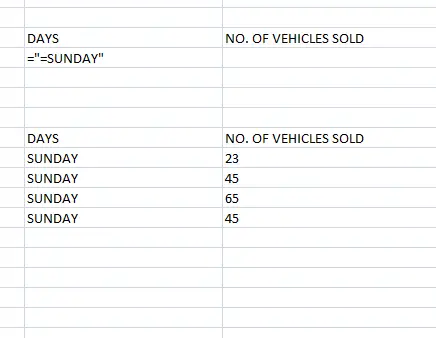
Click OK.
The data will be filtered and will only show the enteries fulfilling the conditions given.
HOW TO ENTER MULTIPLE CONDITIONS IN ADVANCED FILTER IN EXCEL?
MULTIPLE CONDITION
In the previous example, we learned the way to apply a single condition to filter the data. Let us learn to apply the multiple conditions too.
In the first case, we put the formula in the DAYS column to show only the SUNDAY vehicle list.
Now we want the SUNDAY where the sale was >40. So we put the condition under the Second column and repeat the procedure mentioned before.
For the criterion, we’ll put the conditions under both the headings as shown in the picture below and repeat the steps.
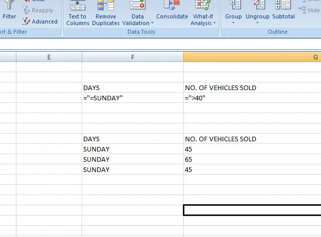
The following picture shows the Result.
We can see that the cases when more than 40 vehicles are sold on SUNDAY are enlisted.
These were the ways to make use of ADVANCED FILTERING in Excel.
FAQs
HOW EXCEL FILTER REMOVES THE UNWANTED DATA?
EXCEL FILTER doesn’t remove the unwanted data but simply hides the lines which doesn’t fulfil the conditions. You can copy this filtered data and paste somewhere else.
WHY THE RESULT DIDN’T UPDATE WHEN I CHANGED THE CONDITIONS IN ADVANCED FILTER IN EXCEL?
ADVANCED FILTER is not a dyanamically controlled process.
It is a one time process.
If you want to refresh the result, simply go to the DATA TAB and click ADVANCED FILTER. The conditions are already filled in. [ If you have already applied it to the data].
Click OK again.
The refreshed data as per the new conditions will be furnished by the EXCEL.
HOW TO CLEAR OR REMOVE ADVANCED FILTER IN EXCEL?
Go to DATA TAB and click CLEAR button just above the ADVANCED FILTER BUTTON.
It’ll remove the ADVANCED FILTER immediately.
IF YOU TRY TO REMOVE THE ADVANCED FILTER BY REMOVING THE RANGES IN THE ADVANCED FILTER SETTINGS BOX, YOU'LL FAIL TO DO SO.
If you don’t want to remove the filter completely but keep a few setting, you can follow the given steps.
Follow the steps in the sequence to remove the advanced filter in Excel but keep the RANGE settings. [ It is as good as removing the filter completely.
- Go to DATA TAB and click ADVANCED FILTER button. The ADVANCED FILTER SETTINGS dialog box will open.
- Delete the CRITERIA RANGE. [Don’t remove the other data. There is no need]
- Click OK.
The filter is removed.
As the filter is removed the complete data will start showing.
You can delete the CRITERIA TABLE if you want.
WHAT IS THE KEYBOARD SHORTCUT TO APPLY ADVANCED FILTER?
Type sequentially ALT+A+Q and the advanced filter setting dialog box will open.