Table of Contents
- INTRODUCTION
- BUTTON LOCATION OF AUTOMATICALLY CREATE PIVOT TABLE IN EXCEL
- BENEFITS OF QUICKLY CREATE A PIVOT TABLE
- STEPS TO USE RECOMMENDED PIVOT TABLES IN EXCEL
INTRODUCTION
PIVOT TABLE is a well known feature of EXCEL which everybody of us might have heard of. But many times we don’t know how to effectively use the PIVOT TABLE.
We have already discussed HOW TO CREATE A PIVOT TABLE AND USE ITS DIFFERENT FUNCTIONS HERE.
Although pivot table creation takes very less time but what if we want it in lesser time .
So we will discuss a really quick way here to create a pivot table automatically in excel or automatic creation of pivot table in excel.
This can be created by an option called RECOMMENDED PIVOT TABLES.
This option , when used , present a number of already made pivot tables which saves us some time by saving us from setting up the fields for the pivot tables. Let us find out more details about the same.
BUTTON LOCATION OF AUTOMATICALLY CREATE PIVOT TABLE IN EXCEL
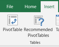
We will find the option for automatically create PIVOT TABLES in EXCEL under the INSERT TAB in TABLES SECTION as shown in the picture below.

BENEFITS OF QUICKLY CREATE A PIVOT TABLE
We know the benefits of PIVOT TABLES.
But here are the benefits of AUTO CREATE PIVOT TABLES.
Most of the times, we have standard situations. We have a data put in the columns having the headings . There are multiple types of data such as numbers and text.
So, what if we get some already created layouts from which we can choose.It is going to be great for sure!So, this is the reason why we can use this function and save us some time.
STEPS TO USE RECOMMENDED PIVOT TABLES IN EXCEL
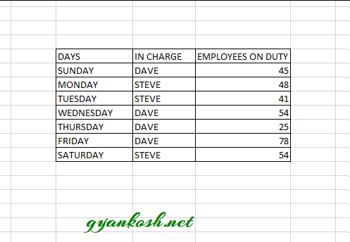
It is always easy to learn a feature using the example.Let us take a simple range from which we will create a pivot table.The data is given below.
| DAYS | IN CHARGE | EMPLOYEES ON DUTY |
| SUNDAY | DAVE | 45 |
| MONDAY | STEVE | 48 |
| TUESDAY | STEVE | 41 |
| WEDNESDAY | DAVE | 54 |
| THURSDAY | DAVE | 25 |
| FRIDAY | DAVE | 78 |
| SATURDAY | STEVE | 54 |

STEPS TO CREATE A PIVOT TABLE:
- Select the data including headers ,go to insert tab and click RECOMMENDED PIVOT TABLES.

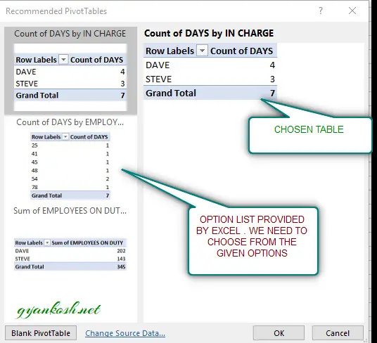
- Click RECOMMENDED PIVOT TABLES BUTTON. A dialog box will open as shown in the following pic.

- The dialog box shown above, is giving the options of the PIVOT TABLES thought of automatically by Excel.
- We need to choose the option from the given ones, which suit us most.
- If none of the option suits us, click BLANK PIVOT TABLE at the bottom of the DIALOG BOX.
- It’ll take us to the standard process of PIVOT TABLE CREATION.
- If we have selected the PIVOT TABLE from the option list, click it.
- It’ll start showing in the right portion of the dialog box as mentioned in the picture above.
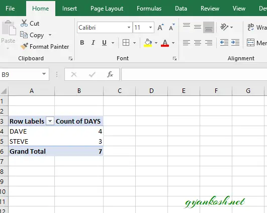
- CLICK OK.
- Our PIVOT TABLE is ready.

After the pivot table is created automatically, we still have complete control over the table.
We can add or remove any fields as per requirement.
FOR MORE INFORMATION ABOUT PIVOT TABLES. CLICK HERE.