Table of Contents
- INTRODUCTION
- PURPOSE OF RANK FUNCTION IN EXCEL
- PREREQUISITES TO LEARN RANK FUNCTION
- SYNTAX: RANK FUNCTION
- EXAMPLES:RANK FUNCTION IN EXCEL [WITH DESCENDING ORDER ]
INTRODUCTION
The RANK function does exactly the same task what its name suggests.
The RANK FUNCTION is found under the STATISTICAL CATEGORY of functions in Microsoft EXCEL.
THE RANK FUNCTION HELPS US TO FIND THE RANK [ POSITION IN A CLASS ] OF ANY NUMBER IN A GROUP OF NUMBERS.
The Rank is same as the position if the numbers are in the descending order. [ If we give the Rank 1 for the highest value].
But what if the numbers given are not in ascending or descending order. In that case, this function will be of immense help.
In this article, we will learn about the purpose, syntax formula, example and other information about the RANK FUNCTION in Excel.
PURPOSE OF RANK FUNCTION IN EXCEL
RANK FUNCTION returns the relative position of the number , by its value, from a group of given numbers.
For example,
Suppose, we have the following numbers.
100,4,2,5,7
Out of these, if we go by the standard rules,
RANK 1 FOR THE HIGHEST VALUE,
Rank 1 will be given to 100.
Rank 2 for 7
Rank 3,4,5 for 5,4 and 2 respectively.
EXCEL GIVES US THE OPTION TO FIND OUT THE RANK IN THE REVERSE WAY TOO [ REFER EXAMPLE BELOW]
PREREQUISITES TO LEARN RANK FUNCTION
THERE ARE A FEW PREREQUISITES WHICH WILL ENABLE YOU TO UNDERSTAND THIS FUNCTION IN A BETTER WAY.
- Basic understanding of how to use a formula or function.
- Basic understanding of rows and columns in Excel.
- Some information about the RANK WORD is an advantage for the use of such formulas.
- Of course, Excel software.
Helpful links for the prerequisites mentioned above
What Excel does? How to use formula in Excel?
SYNTAX: RANK FUNCTION
The Syntax for the RANK function is
RANK ( NUMBER WHOSE RANK TO BE FOUND , REFERENCE , ORDER )
NUMBER WHOSE RANK IS TO BE FOUND This is the number whose rank we want to find.
RANGE This is the group of numbers or class in which we want to find the rank.
ORDER [OPTIONAL] Order on the basis of which RANKING will be done.
If 0 or omitted, Order will be standard. Ranking on the basis of descending values which means HIGHER VALUE will have LOWER RANK.
If 1, Order will be in Reverse. Ranking will be on the basis of ascending values which means LOWER VALUE will have LOWER RANK.
EXAMPLES:RANK FUNCTION IN EXCEL [WITH DESCENDING ORDER ]
EXAMPLE TYPE 1: FIND OUT THE RANK OF THE GIVEN NUMBER
Let us take a group of various numbers.
WE HAVE TAKEN NUMBERS IN A COLUMN, BUT YOU CAN TAKE A COMPLETE TABLE OF NUMBERS TOO.
| 93 |
| 27 |
| 62 |
| 82 |
| 92 |
| 92 |
| 100 |
| 56 |
| 7 |
| 51 |
| 89 |
| 6 |
| 11 |
| 8 |
| 41 |
| 80 |
| 11 |
| 5 |
| 56 |
| 92 |
| 17 |
| 53 |
| 43 |
| 20 |
| 60 |
STEPS TO SUBSTITUTE WORDS IN THE GIVEN TEXT:
- Select the cell where we want the result.
- Enter the formula =RANK(Number, whose rank is to be found, Range , Order).
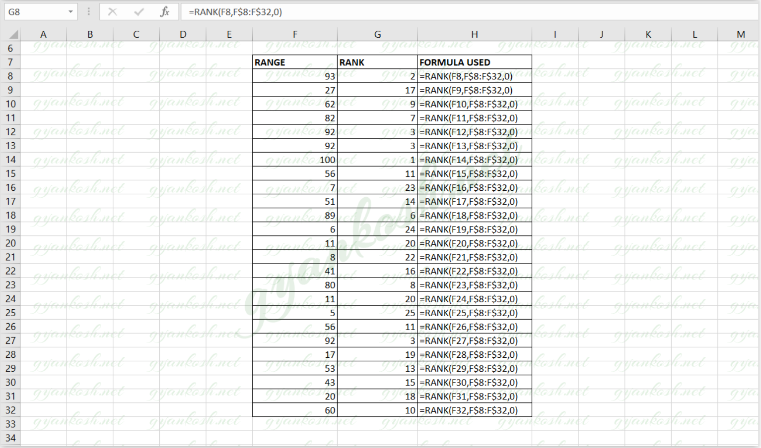
- For our example, the formula will be =RANK(F8,F$8:H$32,0) for the first example.
- Drag down the formula through the column. The results will appear in the respective column.
- The formula used is shown for the help for every example.

EXPLANATION:
The formula used is
=RANK(F8,F$8:H$32,0)
The first argument is F8 which contains the value 93
[ The number of which rank is to be found ].
The second argument is the complete ABSOLUTE RANGE of the group of numbers in which the rank is to be found. We used the absolute range to avoid messing up while dragging down the formula.
The third argument is used to tell the function to FIND OUT THE RANKING FROM THE TOP i.e.From the highest value to the lowest.
We can see that the highest value is given the lowest Rank which is
1.Similarly the lowest value is given the last rank.ONE POINT TO BE REMEMBERED IS THAT
EQUAL VALUES ARE GIVEN SAME RANK, BUT THE NEXT RANK WOULD START AFTER THE NUMBER OF EQUAL RANKS.
To understand the above statement,
let us take a group of numbers. 11, 8,8 6,3
Rank 1 11
Rank 2 8,8
Rank 4 6
Rank 5 3
So, the point should be clear from the above example.
There is not rank 3, as Rank 2 has two 8s.
EXAMPLE TYPE 2: RANKING NUMBERS IN REVERSE ORDER IN EXCEL
In this step, we would try to find the ranking in the reverse order which is, Lower value would be having the Lower rank or we can say just like the Ascending order.
For the Example, let us take a sample of numbers.
| 35 | 41 | 27 |
| 48 | 26 | 24 |
| 24 | 44 | 49 |
| 35 | 23 | 50 |
| 47 | 38 | 23 |
| 39 | 35 | 26 |
| 37 | 48 | 42 |
| 32 | 49 | 27 |
STEPS TO FIND OUT THE RANK OF A NUMBER IN REVERSE ORDER
- Select the cell where we want the result.
- Enter the formula =RANK(Number, whose rank is to be found, Range , Order).
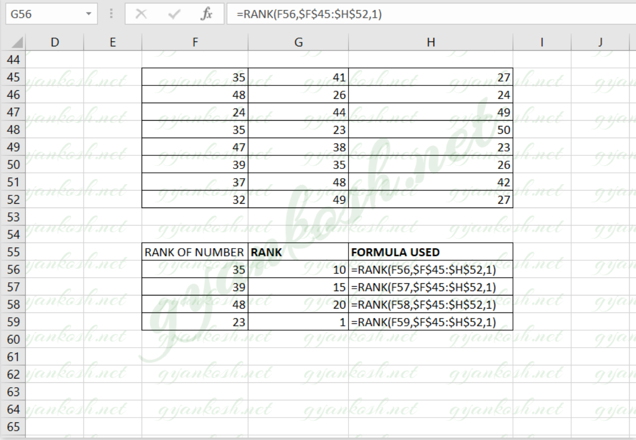
- For our example, the formula will be =RANK(F56,$F$45:$H$52,1) for the first example.
- Drag down the formula through the column. The results will appear in the respective column.
- The formula used is shown for the help for every example.

EXPLANATION:
The function used for the solution is =RANK(F56,$F$45:$H$52,1)
The first argument is F56 which contains the value 35 [ The number of which rank is to be found ].
The second argument is the complete ABSOLUTE RANGE of the group of numbers in which the rank is to be found.
We used the absolute range to avoid messing up while dragging down the formula.
The third argument is used to tell the function to FIND OUT THE RANKING FROM THE BOTTOM i.e. from the last value.
The only difference in this method, from the previous one is the introduction of the ORDER argument which is put in the third place.
The order ID used is 1, which makes the function to RANK the numbers in the Reverse Order.