Table of Contents
- INTRODUCTION
- PURPOSE OF XMATCH IN EXCEL
- PREREQUISITES TO LEARN XMATCH
- WHAT IS THE SYNTAX OF XMATCH IN EXCEL?
- EXAMPLE 1: XMATCH IN EXCEL
- EXAMPLE 2: XMATCH IN EXCEL (SEARCHING THE INDEX IN GIVEN ARRAY)
- EXAMPLE 3: XMATCH IN EXCEL ( FINDING OUT THE NUMBER OF VALUES GREATER OR SMALLER THAN A FIXED VALUE )
- EXAMPLE 4 : WHAT IS FORWARD AND REVERSE SEARCH IN XMATCH ?
- FAQs
- IS XMATCH AVAILABLE IN EXCEL 2013,2016 OR 2019?
- IS XMATCH BETTER THAN MATCH FUNCTION?
INTRODUCTION
XMATCH FUNCTION is a new function introduced in some of the EXCEL VERSIONS, such as EXCEL 365, EXCEL FOR ANDROID ETC.
XMATCH FUNCTION searches for a specified item in a range of cells and returns the relative position.
XMATCH FUNCTION can be used in many ways and for many purposes which are discussed later in this article.
This function is not available in standard Excel application for desktop yet. May be , in future it gets included in that.
PURPOSE OF XMATCH IN EXCEL
XMATCH FUNCTION searches for a specified item in a range of cells and returns its relative position.
“Relative position is the position of any item with respect to the selected range”
PREREQUISITES TO LEARN XMATCH
THERE ARE A FEW PREREQUISITES WHICH WILL ENABLE YOU TO UNDERSTAND THIS FUNCTION IN A BETTER WAY.
- Basic understanding of how to use a formula or function.
- Easier to understand if user already knows how to use MATCH.
- Basic understanding of rows and columns in Excel.
- Of course, Excel software.
Helpful links for the prerequisites mentioned above What Excel does? How to use formula in Excel?
WHAT IS THE SYNTAX OF XMATCH IN EXCEL?
The syntax ( the way how formula is phrased for excel) of XMATCH is
=XMATCH(VALUE TO BE FOUND , LOOKUP TABLE , MATCH MODE , SEARCH MODE )
VALUE TO BE FOUND The value to be found and matched
LOOKUP TABLE The range of cells, where we will try to find the match
MATCH MODE (optional default value=1)
0 – Exact match. If none found, return #N/A. This is the default.
-1 – Exact match. If none found, return the next smaller item.
1 – Exact match. If none found, return the next larger item.
2 – A wildcard match where *, ?, and ~ have special meaning.
SEARCH MODE (optional default=1)
1 – Perform a search starting at the first item. This is the default.
-1 – Perform a reverse search starting at the last item.
2 – Perform a binary search that relies on LOOKUP VALUE being sorted in ascending order. If not sorted, invalid results will be returned.
-2 – Perform a binary search that relies on LOOKUP VALUE being sorted in descending order. If not sorted, invalid results will be returned.
*Binary search is a computer algorithm for the searching fast. But the items should be sorted, which is a pre requisite for this sorting.
EXAMPLE 1: XMATCH IN EXCEL
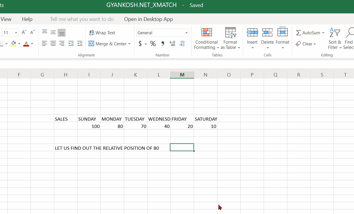
DATA SAMPLE
The example contains the sales number on the weekdays.
The XMATCH function can be used in different ways. Let us first try to use it in the simplest way.
In this example, we will try to find out the relative position of a particular value.
The data contains the different sale numbers as follows.
We’ll find out the relative position of 80.
STEPS TO USE XMATCH – EXAMPLE 1
1. Place the cursor in the cell where we want to get the result.
2. Type the formula
=XMATCH(80,I7:N7,1) (I7 to N7 is the range selected)
3. Click ENTER and the result will appear as 2
EXPLANATION OF STEPS- EXAMPLE 1
The formula used is
=XMATCH(80,I7:N7,1)
80 is the value to be found.
I7:N7 is the range, in which the value is to be found.
1 is the MATCH MODE which will return the next largest number if the number is not found.
FOURTH ARGUMENT IS OPTIONAL WHICH WE WILL USE IN LATER IN THIS ARTICLE.
EXAMPLE 2: XMATCH IN EXCEL (SEARCHING THE INDEX IN GIVEN ARRAY)
DATA SAMPLE
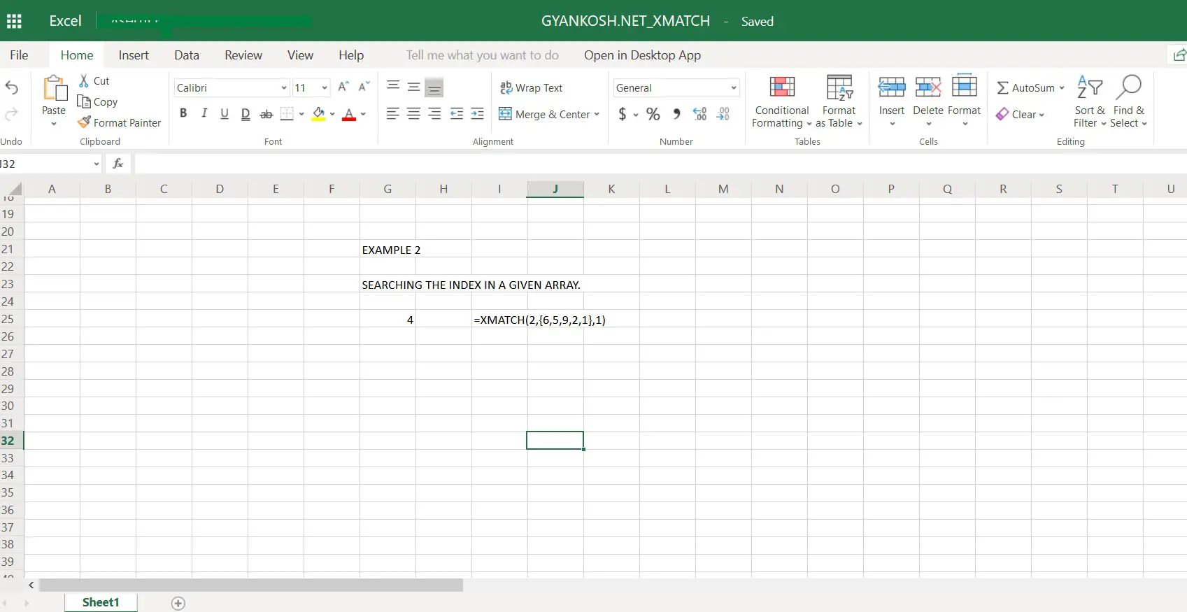
In this example, we will find the index of any element in a given array.
Suppose the array is given as
{6,5,9,2,1}
This array is directly used.
In this example we’re going to get the index/position of element 2.
STEPS TO USE XMATCH – EXAMPLE 2
This is one step formula.
1. Place the cursor in the cell where we want the result.
2. Put the following formula in the cell
=XMATCH(2,{6,5,9,2,1},1)
3. The answer will appear as 4, which is evident as 2 is at the fourth place in the array.
EXPLANATION OF STEPS- EXAMPLE 2
The formula used is
=XMATCH(2,{6,5,9,2,1},1)
The first value is the VALUE TO BE FOUND.
Second argument is the array, in which the value is to be found.
Third argument is the MATCH MODE, which is 1, which will search the match and if not found next higher value will be taken.
Fourth argument is optional which will be seen in EXAMPLE 4.
EXAMPLE 3: XMATCH IN EXCEL ( FINDING OUT THE NUMBER OF VALUES GREATER OR SMALLER THAN A FIXED VALUE )
DATA SAMPLE
In this example, we’ll try to use XMATCH to find out the number of values
greater than or smaller than a particular value. The example finds out the number of values greater than 75 which is a fixed value.
The given range is having the following values.
*The table won’t be visible in mobiles. Its same as shown in the animated picture.
| 1. DAYS | SALES | FIXED VALUE | |
| SUNDAY | 100 | ||
| MONDAY | 80 | 75 | |
| TUESDAY | 70 | ||
| WEDNESDAY | 40 | ||
| FRIDAY | 20 | ||
| SATURDAY | 10 |
Let us try to use XMATCH to find out the number of values greater than 75.
*The data needs to be in descending order, else formula will malfunction.

STEPS TO USE XMATCH – EXAMPLE 3
1. Place the cursor in the cell where we want the result.
2. Put the following formula in the cell
=XMATCH(J38,I36:N36,1)
3. The answer will appear as 2, as we can see that there are only two values greater than 75.
EXPLANATION OF STEPS- EXAMPLE 3
The formula used is
=XMATCH(J38,I36:N36,1)
The first reference is J38 which corresponds to the fixed value which is 75.
Second argument is the range under examination from which we need to extract the output.
Third argument is the MATCH MODE which is 1, which will do the real job in this case.
As MATCH MODE 1 will return the value index or the next largest value, it gives the answer as 2 as the value greater than 75 is 2. (value is 80).
EXAMPLE 4 : WHAT IS FORWARD AND REVERSE SEARCH IN XMATCH ?
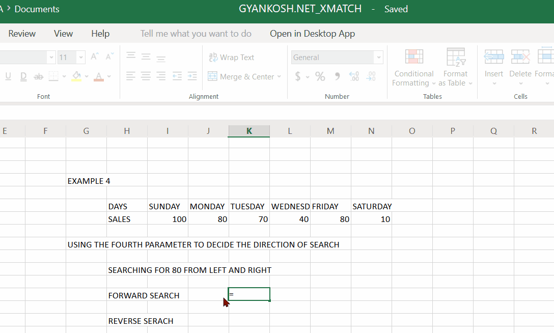
DATA SAMPLE
LET US NOW TRY SOME OPTIONS WITH THE FOURTH ARGUMENT.We will use the two options 1 and -1 which specifies the direction of search i.e. forward search and reverse search.The taken data is same as the previous examples*The table won’t be visible in mobiles. Its same as shown in the animated picture.
| EXAMPLE 4 | |
| DAYS | SALES |
| SUNDAY | 100 |
| MONDAY | 80 |
| TUESDAY | 70 |
| WEDNESDAY | 40 |
| FRIDAY | 80 |
| SATURDAY | 10 |
LET US TRY TO FIND OUT THE INDEX OF VALUE 80 WHICH IS PRESENT AT TWO PLACES IN THE DATA.
STEPS TO USE XMATCH – EXAMPLE 4
1. Place the cursor in the cell where we want to get the result.
FORWARD SEARCH:
2. Type the formula
=XMATCH(J48,I48:N48,1,1)
3. Click ENTER and the result will appear as 2.
REVERSE SEARCH:
=XMATCH(J48,I48:N48,1,-1)
4. Click ENTER and the result will appear as 5.
EXPLANATION OF STEPS- EXAMPLE 4
FORWARD SEARCH:
The formula used is
=XMATCH(J48,I48:N48,1,1)
The first reference is the value to be searched for.
Second argument is the range in which the value is to be found.
Third argument is the MATCH MODE which is 1. i.e. find the value or the next largest number.
Fourth argument is the SEARCH MODE and 1 means forward search.
The excel will search from left to right.
The answer appears as 2, as 80 appears at position 2 when searched from the left.
REVERSE SEARCH:
The formula used is =XMATCH(J48,I48:N48,1,-1)
The first reference is the value to be searched for.
Second argument is the range in which the value is to be found.
Third argument is the MATCH MODE which is 1. i.e. find the value or the next largest number.
Fourth argument is the SEARCH MODE and 1 means forward search. The excel will search from left to right.
The answer appears as 5, as 80 appears at position 5 when searched in reverse.
FAQs
IS XMATCH AVAILABLE IN EXCEL 2013,2016 OR 2019?
No, XMATCH is only avalable for OFFICE 365 [ or EXCEL 365].
IS XMATCH BETTER THAN MATCH FUNCTION?
Yes, XMATCH is a better version of MATCH Function.