INTRODUCTION
You must have come across a scenario when you were summing up a big number of rows but the sum didn’t appear but error. After that you started searching for the errors and ignoring them or improving them.
Here comes the remedy for such cases- The AGGREGATE FUNCTION.
AGGREGATE function comes under the Math&Trig category in Excel.
This function was introduced in Excel 2010 and is available in all versions after that.
AGGREGATE FUNCTION returns the aggregate (sum or conditional operation’s total) of a given list or database with the option of ignoring errors or hidden rows and a number of other options.
This function is really beneficial in practical situations where we need to handle the situations with errors. Most of other functions fail in such situations but Aggregate function still returns the answer.
PURPOSE OF AGGREGATE FUNCTION IN EXCEL
AGGREGATE FUNCTION returns the aggregate (sum or conditional operation’s total) of a given list or database with the option of ignoring errors or hidden rows and a number of other options.
PREREQUISITES TO LEARN AGGREGATE FUNCTION
THERE ARE A FEW PREREQUISITES WHICH WILL ENABLE YOU TO UNDERSTAND THIS FUNCTION IN A BETTER WAY.
- Basic understanding of how to use a formula or function.
- Basic understanding of rows and columns in Excel.
- Some information about the financial terms is an advantage for the use of such formulas.
- Of course, Excel software.
Helpful links for the prerequisites mentioned aboveWhat Excel does? How to use formula in Excel?
SYNTAX: AGGREGATE FUNCTION
There are two types of SYNTAX for AGGREGATE FUNCTION
SYNTAX 1: ARRAY FORM
AGGREGATE(function_num, options, array, [k])
function_num is the FUNCTION given by a number. The table is shown below.
options Choice of options during the operations such as ignoring the errors etc. Given by a number. Table is given below.
array The data on which function will be applied
k[optional] It is used in few listed function e.g. LARGE, SMALL etc. where we need the kth large number or kth small number etc.
SYNTAX 2: REFERENCE FORM
AGGREGATE(function_num, options, ref1, ref2, …)
function_num is the FUNCTION given by a number. The table is shown below.
options Choice of options during the operations such as ignoring the errors etc. Given by a number. Table is given below.
ref1,ref2.. are the references which are to be operated by the selected function. e.g. a1:a14 or individual data can be passed on etc.
LIST OF FUNCTIONS ARGUMENT TO USE IN AGGREGATE FUNCTION
HERE IS THE LIST OF FUNCTION AND THEIR CODE TO BE USED IN AGGREGATE FUNCTION. PUT THE NUMBER IN THE FIRST ARGUMENT OF THE AGGREGATE FUNCTION.
| Function_num | Function |
|---|---|
| 1 | AVERAGE |
| 2 | COUNT |
| 3 | COUNTA |
| 4 | MAX |
| 5 | MIN |
| 6 | PRODUCT |
| 7 | STDEV.S |
| 8 | STDEV.P |
| 9 | SUM |
| 10 | VAR.S |
| 11 | VAR.P |
| 12 | MEDIAN |
| 13 | MODE.SNGL |
| 14 | LARGE |
| 15 | SMALL |
| 16 | PERCENTILE.INC |
| 17 | QUARTILE.INC |
| 18 | PERCENTILE.EXC |
| 19 | QUARTILE.EXC |
LIST OF OPTION ARGUMENT TO USE IN AGGREGATE FUNCTION
HERE IS THE LIST OF OPTION NUMBER TO BE USED IN AGGREGATE FUNCTION. PUT THE NUMBER IN THE SECOND ARGUMENT OF THE AGGREGATE FUNCTION.
| Option | Behavior |
|---|---|
| 0 or omitted | Ignore nested SUBTOTAL and AGGREGATE functions |
| 1 | Ignore hidden rows, nested SUBTOTAL and AGGREGATE functions |
| 2 | Ignore error values, nested SUBTOTAL and AGGREGATE functions |
| 3 | Ignore hidden rows, error values, nested SUBTOTAL and AGGREGATE functions |
| 4 | Ignore nothing |
| 5 | Ignore hidden rows |
| 6 | Ignore error values |
| 7 | Ignore hidden rows and error values |
EXAMPLE 1:AGGREGATE FUNCTION IN EXCEL
DATA SAMPLE
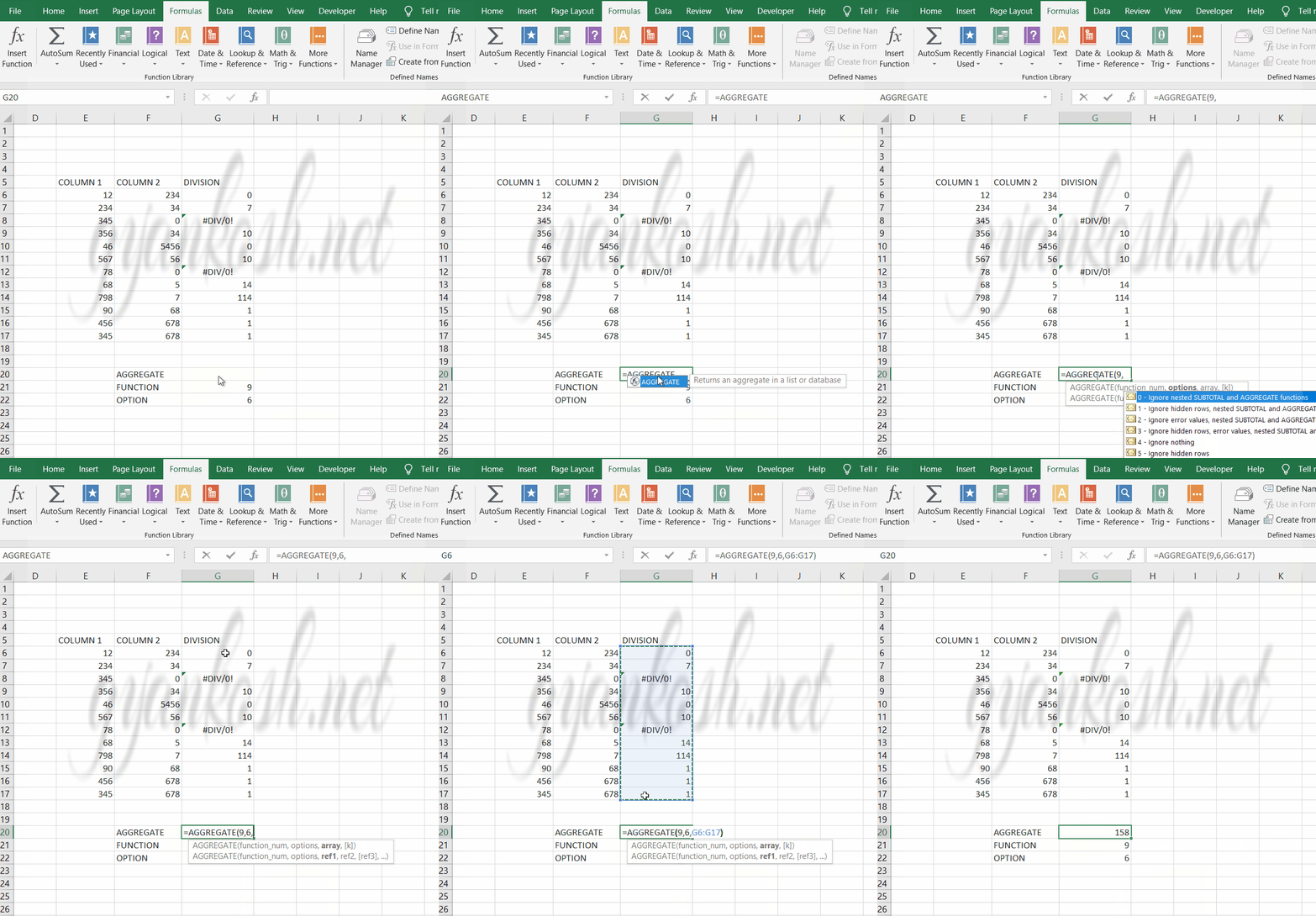
We’ll take a few examples to try this AGGREGATE FUNCTION.Let us take two columns of numbers, where we’d divide the first column from the second and find out the SUM of the third column using AGGREGATE FUNCTION. The third column will be having some errors which we will create intentionally and check the efficacy of this function.The data is as follows.
| COLUMN 1 | COLUMN 2 | DIVISION |
| 12 | 234 | 0 |
| 234 | 34 | 7 |
| 345 | 0 | #DIV/0! |
| 356 | 34 | 10 |
| 46 | 5456 | 0 |
| 567 | 56 | 10 |
| 78 | 0 | #DIV/0! |
| 68 | 5 | 14 |
| 798 | 7 | 114 |
| 90 | 68 | 1 |
| 456 | 678 | 1 |
| 345 | 678 | 1 |
CREATION AND RUNNING OF THE EXAMPLE 1

STEPS TO USE AGGREGATE FUNCTION
We have two columns and the third column contains the result of the division of two columns.
We can see that the third column has a few errors. Still we want to sum these up.
If we use simple SUM function, it’ll return an error. So we use the following function
=AGGREGATE(9,6,G6:G17)
9 is the code of SUM FUNCTION
6 is the option given to ignore error values.
and G6:G17 is the range to be summed up.
The answer comes out to be 158 which is correct.
Similarly we can use any function.
Let us take one example with the k option.
xlChart has the following values. We can use the name as well as value. Kindly read them once.
Specifies the chart type.
EXAMPLE 2:AGGREGATE FUNCTION IN EXCEL USING K ARGUMENT
DATA SAMPLE
We already discussed a simple example of the aggregate function but we omitted the last argument. Now let us take another example where we need the fourth argument too.
We’ll take a few examples to try this AGGREGATE FUNCTION.
Let us have a data and we’ll find out the second highest number in the data.
We’ll put some intentional errors in this range.
The range is following
| RANGE 1 |
| 12 |
| 67 |
| 23 |
| 34 |
| 45 |
| 56 |
| 243 |
| #DIV/0! |
| 123 |
| 23 |
| 213 |
| 2 |
| 12 |
CREATION AND RUNNING OF EXAMPLE 2

STEPS TO USE AGGREGATE FUNCTION- EXAMPLE 2
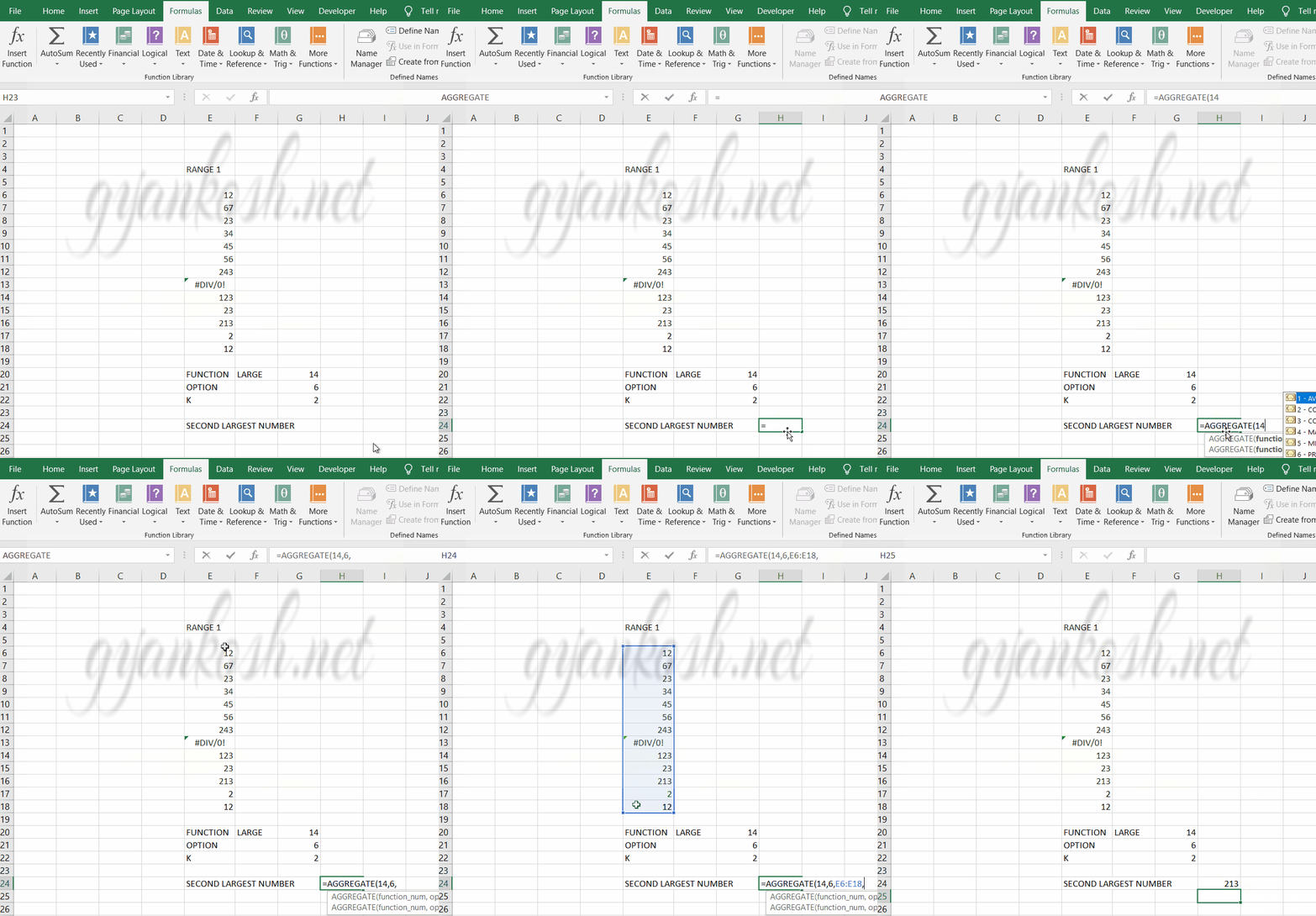
We have a range in this example.
The range consists of different numbers randomly placed and one of the value is having error too.
We’ll find the second largest number from this range using the AGGREGATE FUNCTION.
So we use the function as
=AGGREGATE(14,6,E6:E18,2)
14 is the code for LARGE FUNCTION. Refer the table above.
6 is the option for ignoring the error values. Refer table above.
E6:E18 is the range
2 is the kth number.