Table of Contents
- INTRODUCTION
- What is the use of Address Function in Excel?
- PREREQUISITES TO LEARN ADDRESS
- How to write Address function in Excel? (Syntax of Address Function)
- EXAMPLES : Using ADDRESS FUNCTION IN EXCEL
INTRODUCTION
In this article, we’ll learn about the Address function in Excel.
ADDRESS function comes under the LOOKUP AND REFERENCE category in Excel.
ADDRESS FUNCTION returns the address of any cell which is specified by the ROW number and COLUMN number.
It gives us the option of simple calculation of Row number and Column number as it is cumbersome to handle the column names after Z.
This function also gives additional option of setting which type of ADDRESS we want. A1 type or R1C1 type. A1 type is the standard system of naming where row is shown using a number and column is marked using an Alphabet.
Whereas in R1C1 method , both row and column are shown using numbers.
In this article, we’ll learn to use the ADDRESS FUNCTION, its purpose, formula syntax and various examples for the clarification purpose.
What is the use of Address Function in Excel?
ADDRESS FUNCTION returns the cell address in a specified format when we pass the row and column number as arguments. It is often used when you need to dynamically generate cell references in formulas, especially when working with data that changes or shifts.
Address function can be used for the following cases:
Dynamic references: You can combine the ADDRESS function with other functions like MATCH or ROW to generate dynamic cell references in a formula.
Working across sheets: The sheet_text argument allows you to reference cells in other worksheets.
Customizable references: It lets you switch between absolute, relative, and mixed references depending on your need.
PREREQUISITES TO LEARN ADDRESS
THERE ARE A FEW PREREQUISITES WHICH WILL ENABLE YOU TO UNDERSTAND THIS FUNCTION IN A BETTER WAY.
- Basic understanding of how to use a formula or function.
- Basic understanding of rows and columns in Excel.
- Some information about the financial terms is an advantage for the use of such formulas.
- Of course, Excel software.
Helpful links for the prerequisites mentioned above What Excel does? How to use formula in Excel?
How to write Address function in Excel? (Syntax of Address Function)
The Syntax for the function is
=ADDRESS(ROW NUMBER, COLUMN NUMBER, ADDRESS RETURN TYPE, ADDRESS RETURN STYLE, SHEET NAME )
ROW NUMBER The row number to be used in the cell address
COLUMN NUMBER The column number to be used in the cell address.
ADDRESS RETURN TYPE The address can be returned as absolute , relative or mixed. The numbers and their application is shown in the table below.
| ABSOLUTE RETURN TYPE | EFFECT ON THE RETURN TYPE |
|---|---|
| 1 or omitted | Absolute [ e.g. $A$8] |
| 2 | Absolute row; relative column [ e.g. A$8] |
| 3 | Relative row; absolute column [ e.g. $A8] |
| 4 | Relative [ e.g. A8] |
ADDRESS RETURN STYLE We can use the address in two styles in Excel sheets. The style are A1 style and R1C1 style.
A1 is the by default style where first letter shows the COLUMN NAME and second digit shows the ROW NUMBER.
R1C1 style treats both the values as numbers. i.e. the first digit shows the row number whereas the second digit shows the column number.
TRUE or OMITTED means the default style i.e. A1 style whereas
FALSE means the R1C1 style.
SHEET NAME is the name of the sheet we want to include with the address return. It might be need if we want to get the cell address of some other sheet.
The usage will be clarified when we solve the examples given below.
EXAMPLES : Using ADDRESS FUNCTION IN EXCEL
DATA SAMPLE
Let us take a few examples and see how ADDRESS function is working in the given situations.
Following table shows different parameters. We’ll put them in Excel sheet and see what is the output.
| ROW NUMBER | COLUMN NUMBER | RETURN TYPE | RETURN STYLE | SHEET NAME | |
| EXAMPLE 1 | 2 | 4 | 1 | TRUE | SHEET |
| EXAMPLE 2 | 5 | 6 | 2 | TRUE | [BOOK1]!SHEET1 |
| EXAMPLE 3 | 3 | 4 | 3 | FALSE | |
| EXAMPLE 4 | 5 | 6 | 4 | OMITTED | |
| EXAMPLE 5 | 2 | 4 | OMITTED | OMITTED | OMITTED |
| EXAMPLE 6 | 1 | 4 | 2 | 1 |
STEPS TO USE ADDRESS FUNCTION
FOLLOW THE STEPS TO USE ADDRESS FUNCTION IN EXCEL
We have taken various examples to show the use of ADDRESS FUNCTION.
Select the cell where we want to obtain the cell address.
Enter the function as shown in the picture above.
The result will appear in the cell.
NOTE: In the examples, we have used the cells references containing the data. We can use the data directly too.
We can always use 1 in place of TRUE and 0 in place of false. The results will be accurate.
EXPLANATION
We have taken various examples to show the use of ADDRESS FUNCTION.
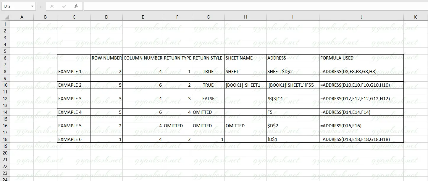
EXAMPLE 1– Use Address function in Excel to return an absolute address with sheet name.
The formula used is =ADDRESS(D8,E8,F8,G8,H8)
Here we have used all the five arguments. It has returned an absolute address with the sheet name.
EXAMPLE 2– Use address function in Excel to return Relative Column and Absolute Row
The formula used is =ADDRESS(D10,E10,F10,G10,H10).
In this example, we have used all the five arguments. This example returned relative column and absolute row, with the workbook and sheet name.
We can see that FIFTH ARGUMENT is simply attached with the address. So always be careful to give it in proper format so that our address is working properly.
EXAMPLE 3– Use Address function in Excel to return address in R1C1 style.
The formula used is =ADDRESS(D12,E12,F12,G12,H12)
We have used all the five arguments in this example but haven’t given any sheet name. The style has been taken as false so that we get the result in R1C1 style. The result is as per expectation.
EXAMPLE 4– Use Address function in Excel to return Relative address.
The formula used is =ADDRESS(D14,E14,F14)
In this example, we used only the first three arguments. The result is simple relative address as per the given arguments.
EXAMPLE 5– Use Address function in Excel to return Absolute Address
The formula used is =ADDRESS(D16,E16)
We have used only the two required arguments and the result is simple absolute address.
EXAMPLE 6– Use Address function in Excel to return Relative column and absolute row
The formula used is =ADDRESS(D18,E18,F8,G18,H18)
NOTE: DID YOU NOTICE AN EXCLAMATION BEFORE THE ADDRESS IN THE EXAMPLES WITH EMPTY ARGUMENT. IT WAS SO BECAUSE WE TOOK AN EMPTY SHEET NAME. IF WE DON’T WANT SHEET NAME, WE SHOULD OMIT IT.