INTRODUCTION
EXCEL provides a complete set of functions to deal with the database data.
DATABASE data has the first row as headers.
DSUM FUNCTION ADDS THE VALUES IN A COLUMN [ FIELD ] WHICH FULFILLS A GIVEN CONDITION.
DSUM function is very useful if we need to find out the sum of data on the basis of any classification which can be changed by changing the condition.
PURPOSE OF DSUM IN EXCEL
DSUM FUNCTION ADDS THE NUMBERS PRESENT IN A COLUMN [ FIELD ] WHICH SATISFIES THE GIVEN CONDITION.
PREREQUISITES TO LEARN DSUM
THERE ARE A FEW PREREQUISITES WHICH WILL ENABLE YOU TO UNDERSTAND THIS FUNCTION IN A BETTER WAY.
- Basic understanding of how to use a formula or function.
- Of course, Excel software.
Helpful links for the prerequisites mentioned aboveWhat Excel does? How to use formula in Excel?
SYNTAX: DSUM FUNCTION
The Syntax for the DSUM function is
=DSUM(database or range, column or field, Criteria )
The DSUM function syntax has the following arguments:
- Database Database is the data on which we want to use the DSUM function. The data is specifically arranged in DATABASE STYLE with LABELS in the top row and data in the lower rows. The range mentioning the database is given including the cells containing the Labels.
- Field Column or field is the column on which the criteria will be applied. The column is given by the column name in the “” or it can be given as the column number of the database such as 1 ,2 and so on.
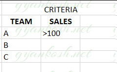
- Criteria It is the range which contains the criteria or conditions. It is important that the range contains the column label. It’ll become clearer with the example discussed below.
EXAMPLE:DSUM FUNCTION IN EXCEL
DATA SAMPLE
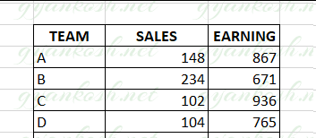
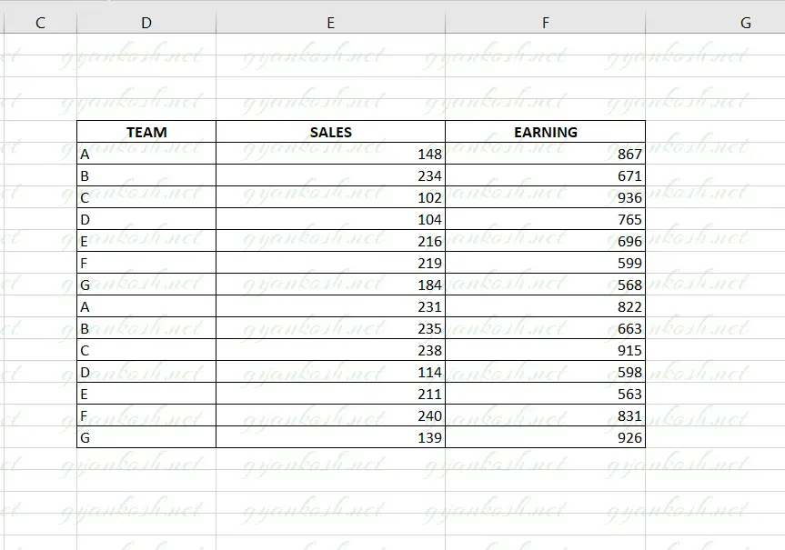
DSUM FUNCTION usage can be a bit confusing for the new learners. For the simplicity let us take an example to understand the Do’s and Don’t of DSUM.We have the following data of Sales teams for two months.The table below shows the data present with us.
| TEAM | SALES | EARNING |
| A | 148 | 867 |
| B | 234 | 671 |
| C | 102 | 936 |
| D | 104 | 765 |
| E | 216 | 696 |
| F | 219 | 599 |
| G | 184 | 568 |
| A | 231 | 822 |
| B | 235 | 663 |
| C | 238 | 915 |
| D | 114 | 598 |
| E | 211 | 563 |
| F | 240 | 831 |
| G | 139 | 926 |
Let us try to find out a few analytical points from the table.1. Find out the total sales by team A.2. Find out the total earning by team C.
1. FINDING OUT THE TOTAL SALES BY TEAM A USING DSUM FUNCTION
Let us try to find out the total sales done by the Team A.
Follow the steps to find out the total sale.
- After we have our data ready i.e. The table must be having the column labels at the top. [ There is no specific requirements for the column labels. The function would consider the first row as column labels. ]
- The criteria needs to be declared as a range. The range must contain atleast one column label at the top followed by the condition under the columns.
- Put the formula in a cell where you want the result
- =DSUM(D5:F19,”SALES”,H5:J6)
- The function returns the result as 379.
- The following animated picture shows the process of using DSUM function in Excel.
The explanation follows the picture below.
EXPLANATION: FINDING OUT TOTAL SALES BY TEAM A
The function used for the solution is
=DSUM(D5:F19,”SALES”,H5:J6)
Let us analyze the formula used.
The first parameter i.e. D5:F19 is the complete range of the Database [data ].
The second parameter “SALES” is the field or column on which the condition would work. As we want to know the total sales, SALES column is needed.
The column is always given in the Double Quotes. [” “].
The last parameter is the range containing the Criteria H5:J6.
Have a look at the way criteria is described. The column names must be same as the database so that the function can lookup and give you the result.
The condition is given below the column.
2. FINDING OUT THE TOTAL EARNINGS MADE BY TEAM C USING DSUM FUNCTION
Let us try to find out the total earnings done by Team C.
Follow the steps to find out the total earnings.
- After we have our data ready i.e. The table must be having the column labels at the top. [ There is no specific requirements for the column labels. The function would consider the first row as column labels. ]
- The criteria needs to be declared as a range. The range must contain atleast one column label at the top followed by the condition under the columns.
- Put the formula in a cell where you want the result
- =DSUM(D5:F19,”EARNING”,H12:J13)
- The function returns the result as 1851.
- The following animated picture shows the process of using DSUM function in Excel.
The explanation follows the picture below.
EXPLANATION: FINDING OUT TOTAL EARNINGS BY TEAM C
The function used for the solution is
=DSUM(D5:F19,”EARNING”,H12:J13)
Let us analyze the formula used.
The first parameter i.e. D5:F19 is the complete range of the Database [data ].
The second parameter “EARNING” is the field or column on which the condition would work. As we want to know the total Earnings, EARNING column is needed.
The column is always given in the Double Quotes. [” “].
The last parameter is the range containing the Criteria H12:J13.
Have a look at the way criteria is described. The column names must be same as the database so that the function can lookup and give you the result.
The condition is given below the column.