Table of Contents
- INTRODUCTION
- PURPOSE OF SUBSTRING EXTRACTION IN GOOGLE SHEETS ?
- CONCEPT: EXTRACT SUBSTRING FROM THE GIVEN TEXT
- GET SUBSTRING FROM VARIOUS POSITIONS IN THE GIVEN TEXT
- EXTRACT SUBSTRING FROM THE BEGINNING [ LEFT ]
- EXTRACT SUBSTRING FROM THE END [ RIGHT ]
- EXTRACT SUBSTRING FROM THE MIDDLE PORTION
- EXTRACT SUBSTRING BEFORE A CERTAIN CHARACTER OR STRING
- EXTRACT SUBSTRING AFTER A CERTAIN CHARACTER OR STRING
- EXTRACT SUBSTRING AFTER A CERTAIN CHARACTER OR STRING
INTRODUCTION
GOOGLE SHEETS is one of the great Spreadsheet applications available today in the market.
The two important components of any reports are the numbers and the text. If you want to be proficient in google sheets, you need to be perfect in handling both text as well as the numbers.
One of such situations arises when we need to extract a substring function in Google Sheets.
THERE IS NO DIRECT FUNCTION TO EXTRACT SUBSTRING FROM THE GIVEN TEXT BUT WE CAN MAKE USE OF A FEW AVAILABLE FUNCTION TO EXTRACT THE SUBSTRING FROM THE GIVEN TEXT IN GOOGLE SHEETS.
In this article, we’d learn to extract a substring from the given text or string in Google Sheets.
PURPOSE OF SUBSTRING EXTRACTION IN GOOGLE SHEETS ?
The requirement to extract a portion of the text may arise any time while creating any reports in Google Sheets.
There can be a few requirements where we need to extract a sub string like
- Extracting a particular portion from a sentence or text.
- Extracting any letters from the text.
- Extract a word from a line.
and many more other possibilities.
CONCEPT: EXTRACT SUBSTRING FROM THE GIVEN TEXT
We can extract a substring in many ways.
We can use our standard LEFT, MID AND RIGHT FUNCTIONS to extract the substring from the cell in GOOGLE SHEETS.
LEFT FUNCTION has the capability to pick the specified number of characters from the left side of the text.
The syntax is =LEFT(CELL CONTAINING TEXT,NUMBER OF CHARACTERS FROM THE LEFT)
RIGHT FUNCTION can extract the specified number of characters from the right whereas
The syntax is =RIGHT(CELL CONTAINING TEXT,NUMBER OF CHARACTERS FROM THE RIGHT)
MID FUNCTION takes out the specified number of the characters from the middle of the text.
The syntax is =MID(CELL CONTAINING TEXT,STARTING POSITION OF THE TEXT TO BE EXTRACTED, NUMBER OF CHARACTERS TO BE EXTRACTED)
EXAMPLES
Let us take a few examples to learn how to extract text from the cell.
GENERALIZED STEPS TO EXTRACT SUBSTRING FROM CELLS:
- Select the cell where we want the result.
- FOR TEXT FROM LEFT: Use LEFT function to extract data from the left. Use the function as =LEFT(CELL CONTAINING TEXT, NUMBER OF CHARACTERS)
- FOR TEXT FROM RIGHT: Use RIGHT function to extract data from the right. Use the function as =RIGHT(CELL CONTAINING TEXT, NUMBER OF CHARACTER)
- FOR TEXT FROM THE MIDDLE PORTION: Use MID function to extract data from anywhere in the TEXT. Use the function as =MID(CELL CONTAINING TEXT, CHARACTER POSITION FROM WHERE THE TEXT PICKING WILL START, NUMBER OF CHARACTERS TO BE EXTRACTED.)
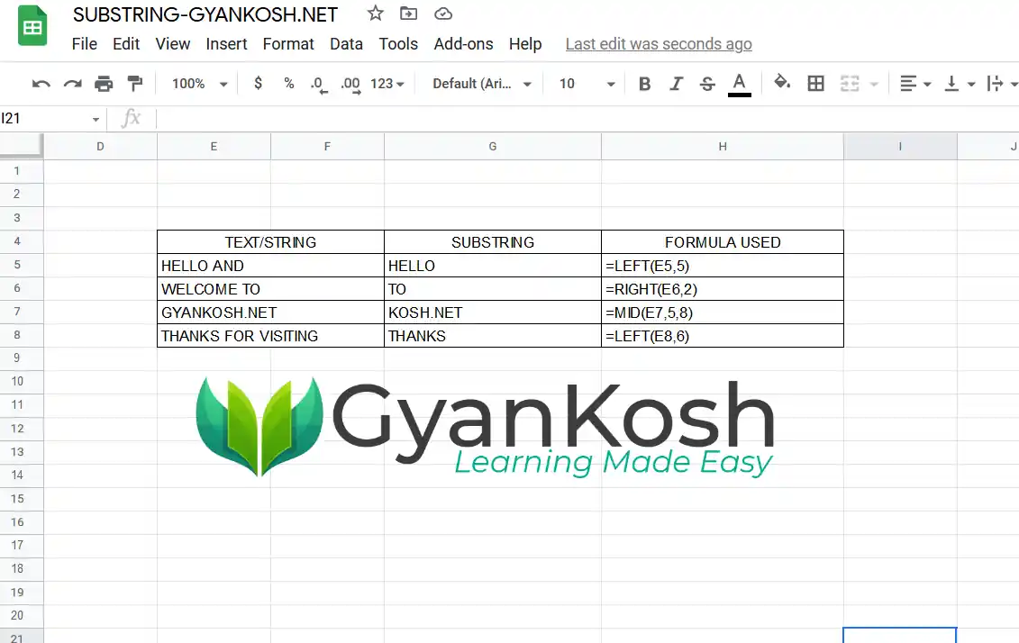
- The Text , Extracted text and formula are shown in the picture below.
- In the following picture we have taken FOUR EXAMPLES by putting the distributed text in the four rows.
- The extraction result is shown and the formula used is shown too. [ Try to solve, if can’t explanation follows the picture below ].
EXPLANATION:
If you look at the picture above we have taken a few examples there to extract the SUBSTRING from the given TEXT.
The sample text is given under the heading TEXT/STRING.
- Extract HELLO from the given text HELLO AND.
We can see that HELLO is the starting word in the sentence [ or rather a group of words].
We can easily extract the word from the given text by using the LEFT FUNCTION.
The formula use is =LEFT(E5,5)
We’ll count the number of character which comes out to be 5 for this case.
2. Extract TO from the given text WELCOME TO.
In this case, we can see that TO is easily accessible from the RIGHT SIDE. So we can easily use the function RIGHT to extract 2 letters from the right direction.
So the formula used as =RIGHT(E6,2) extracts the desired TO from the given text.
3. Extract KOSH.NET from the given text GYANKOSH.NET
In this case, we can see that we need to extract the text from the mid although can be accessed from the Right too.
We’ll make use of MID function to extract this .
The function is used as =MID(E7,5,8)
This formula/function will extract the desired portion KOSH.NET from the text and put it in the result cell.
4. Extract THANKS from the given text THANKS FOR VISITING.
This is again the example of case when we have the easy access from the LEFT.
So we used the simple function LEFT as =LEFT(E8,6)
which will extract the word THANKS from the given text snippet.
So, in this article, we learnt to extract the SUBSTRING from the given text in various ways.
Not just this but this trio [ LEFT, RIGHT , MID ] is extremely simple and powerful at the same time. Whenever we need to get any custom characters from the given text , these functions are every ready to help.
The possibilities are unlimited.
Let us discuss a few simple situations for the easy learning.
GET SUBSTRING FROM VARIOUS POSITIONS IN THE GIVEN TEXT
Let us take the text Welcome to Gyankosh.net and use the discussed functions to extract substring from various positions. [ Some examples are revisited ]
EXTRACT SUBSTRING FROM THE BEGINNING [ LEFT ]
Extract 6 letters from the left:
GIVEN TEXT: “GYANKOSH.NET“
FORMULA TO BE USED: =LEFT(“GYANKOSH.NET”,5)
Result: GYANK
EXTRACT SUBSTRING FROM THE END [ RIGHT ]
Extract 4 letters from the left:
GIVEN TEXT: “GYANKOSH.NET“
FORMULA TO BE USED: =RIGHT(“GYANKOSH.NET”,4)
Result: .NET
EXTRACT SUBSTRING FROM THE MIDDLE PORTION
Extract 3 LETTERS FROM THE 4TH LETTER
GIVEN TEXT: “GYANKOSH.NET“
FORMULA TO BE USED: =MIDDLE(“GYANKOSH.NET”,4,3)
Result: NKO
EXTRACT SUBSTRING BEFORE A CERTAIN CHARACTER OR STRING
GIVEN TEXT: “GYANKOSH.NET“
FORMULA TO BE USED: =LEFT(“GYANKOSH.NET”,SEARCH(“.”,”GYANKOSH.NET”)-1)
Result: GYANKOSH
EXTRACT SUBSTRING AFTER A CERTAIN CHARACTER OR STRING
GIVEN TEXT: “GYANKOSH.NET“
FORMULA TO BE USED: =RIGHT(“GYANKOSH.NET”,LEN(“GYANKOSH.NET”)-SEARCH(“.”,”GYANKOSH.NET”)-LEN(“.”)+1)
Result: NET
EXTRACT SUBSTRING AFTER A CERTAIN CHARACTER OR STRING
GIVEN TEXT: “GYANKOSH.NET“
FORMULA TO BE USED: =RIGHT(“GYANKOSH.NET”,LEN(“GYANKOSH.NET”)-SEARCH(“.”,”GYANKOSH.NET”)-LEN(“.”)+1)
Result: NET
THANKS FOR VISITING.