AVOID ENTERING DUPLICATE VALUES IN A COMPLETE COLUMN OF EXCEL

Table of Contents

• INTRODUCTION
• WHAT IS DATA VALIDATION?
• HOW TO ALLOW ONLY UNIQUE VALUES IN A COLUMN?
  • STEP 1: SELECT THE CELLS
  • STEP 2: APPLY DATA VALIDATION
  • STEP 3: SET ERROR MESSAGE
  • STEP 4: TRIAL RUN

INTRODUCTION

Excel offers a big number of dedicated functionalities which are helpful for us to create many useful applications.

One of such options is Data Validation in Excel.

As we know, data validation helps us to manage the input of the data in the selected cells and condition the input as per our requirement. Data validation can be used to make many conditions viable using the various formulas and options provided through the data validation.

Similarly, in this article, we’ll create one of the frequent and very useful conditions to enter the unique values only in a given column.

WHAT IS DATA VALIDATION?

LEARN THE BASICS OF DATA VALIDATION IN EXCEL.

DATA VALIDATION is the word comprising of two words DATA and VALIDATION.

Data comprises the values whereas validation means validating the input data. Validation means checking the data if it is as per the given conditions or not.

For example, if we want to condition any cell to accept the inputs between 10 and 100, we’ll be able to do this using data validation in excel.

In addition to this, we can provide a list of the options which will populate when the cell is selected. [ DROPDOWN LIST ]

So, these are a few usages of data validation.

You can use the link given above to learn the basics of the DATA VALIDATION in EXCEL which is a must to easily grasp the concepts discussed here.

HOW TO ALLOW ONLY UNIQUE VALUES IN A COLUMN?

Let us try to condition a column in such a way that only the unique values could be entered into this column.

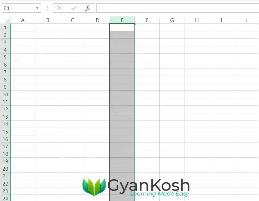
STEP 1: SELECT THE CELLS

Select all the cells where you want to put the condition. In our case, we’ll select a complete column by simply clicking over the column name.

We selected the E COLUMN here and we’ll limit the entries of values in Column E so that only unique values are entered in the E column.

STEP 2: APPLY DATA VALIDATION

After the selection has been made, we need to apply the rules for data validation in Excel.

FOLLOW THE STEPS TO APPLY DATA VALIDATION RULES:

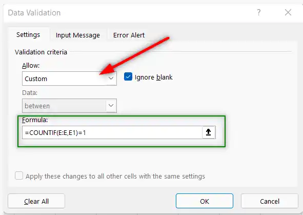
1. After the column is selected, go to DATA TAB and choose DATA VALIDATION button.
2. The following dialog box will open.
3. Choose CUSTOM from ALLOW DROP DOWN LIST marked by a red arrow in the picture below.
4. Enter the formula as =COUNTIF(COLUMN NAME: COLUMN NAME, FIRST REFERENCE )=1.
5. For our example, the formula will be =COUNTIF(E:E,E1)=1.
6. Click OK.

STEP 3: SET ERROR MESSAGE

After setting the formula, we need to set the Error Message. [ Optional ].

FOLLOW THE STEPS TO SET THE ERROR MESSAGE

1. When we have set the formula, choose the ERROR ALERT TAB.
2. Choose STYLE as STOP from the dropdown.
3. Enter the title as DUPLICATE VALUES [ or as per your choice ].
4. Enter the ERROR MESSAGE as THE VALUE ALREADY EXISTS [ or anything as per your choice ].

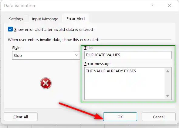
After setting the title and error message, click OK.

STEP 4: TRIAL RUN

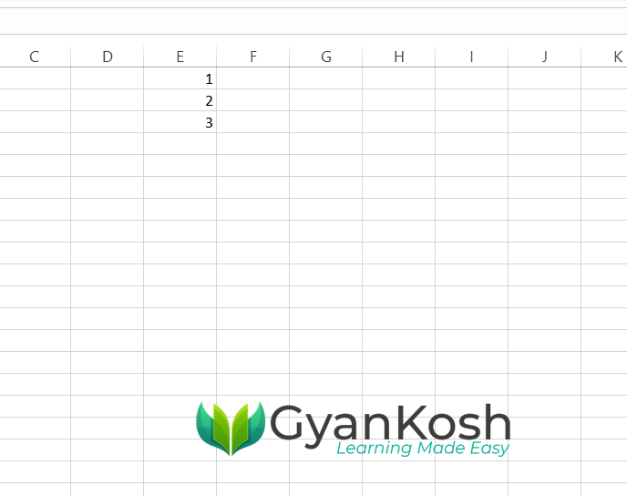
After setting the data validation, let us try to check by entering the repeated values in column E.

We can see that the column is not accepting the repeated values and will show an error alert when any repeated value is added.

We tried to add 3 and 1, which it didn’t allow.

We again entered one text value “asd” and again repeated it by entering “asd” but the value was not accepted.