INTRODUCTION
Sorting is putting up a number of things in a particular fashion as per the selected criteria. Sorting in EXCEL is one of the very basic and frequently used operation.
SORTING IN EXCEL IS THE PROCESS OF ARRANGING THE TEXT OR VALUES SYSTEMATICALLY AS PER THE SELECTED CRITERIA.
WE HAVE ALREADY LEARNT ABOUT THE SORTING DATA IN EXCEL. CLICK HERE TO VISIT. But there can be situations when we want our data to be in the original state. There can be many reasons for that such as
1. We just need to find out any data temporarily and need to come back to the original data.
2. There is some mistake and we haven’t kept any copy of the data.
For these options, let us find out the ways with which we can keep a track and come to the original sequence of the data.
** There can be some confusion about the terminology here.
Unsort or reverse sort used here are specifically meant for the situation when we want to get back to the original state
.If you want to REVERSE THE SORT ORDER OF THE DATA.Click here. [ IDEAS DESCRIBED FOR GOOGLE SHEETS AS OF NOW, BUT CAN BE REFERENCED ]
or
If you want to RANDOMIZE YOUR DATA Click here. [ AVAILABLE FOR GOOGLE SHEETS AS OF NOW, BUT CAN BE REFERENCED ]
WAYS TO REVERSE SORT DATA IN EXCEL
There is no direct option to reverse the sorting of the data in EXCEL .
There are mainly two ways to reverse the sorting.
1. Using the UNDO OPTION.
2. Using the HELPER COLUMN.
UNSORT USING UNDO OPTION
The UNDO OPTION is a life saver in the software or applications as well as in MICROSOFT EXCEL if we performed any action which didn’t result in the outcome as per expectation.
This happens many times while working.
In the case of sorting, it can happen when we need to remove all the steps and get the original data. For that, we can use UNDO OPTION.
The button location for UNDO OPTION is shown in the picture below.
NOTE: THE UNDO OPTION IS AVAILABLE IN THE QUICK ACCESS TOOLBAR WHICH CAN BE PLACED ABOVE THE RIBBON AS WELL AS BELOW THE RIBBON. WE ARE SHOWING THE LOCATION OF THE UNDO REDO OPTIONS AT BOTH THE PLACES.
The following picture shows the button location of UNDO ACTION in EXCEL when the quick access toolbar is placed above the ribbon.
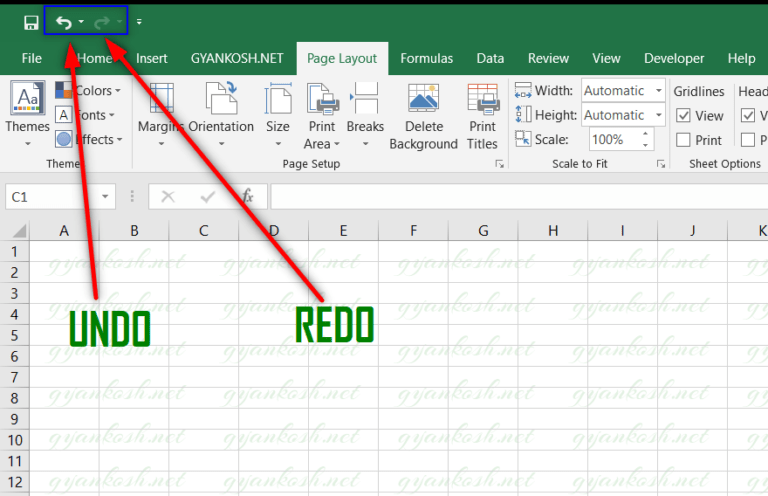
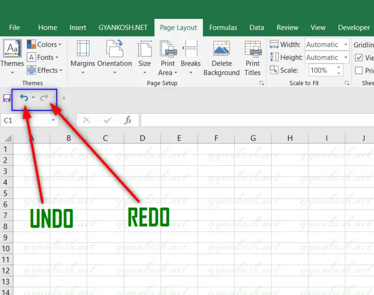
Similarly, the following picture shows the button location of UNDO ACTION when the quick access toolbar is placed below the ribbon.
EXAMPLE:
Let us now learn to use the undo option to reverse the SORT step of any data.
We can make use of the UNDO OPTION in one step or in multi steps as per the requirement.
USING MULTI STEP UNDO:
STEPS TO USE UNDO OPTION:
- Simply press the UNDO BUTTON as shown in the picture above.
- One press will take you ONE OPERATION BACK.
- We can also use KEYBOARD SHORTCUT CTRL+Z for the same. One press means one step back.
- Click UNDO or press CTRL+Z again and again till we get the original unsorted data.
IF, BY MISTAKE, WE REACH THE PREVIOUS STEP OF THE ONE WHERE WE INTENDED TO STOP, WE CAN USE CTRL+Y , OR THE BUTTON NEXT TO UNDO WHICH IS KNOWN AS REDO, TO GO TO THE NEXT STEP.
UNSORT OR REVERSE SORT USING UNDO OPTION [ SINGLE STEP ]
Now, let us take an example to learn the way by which we can reverse all the steps to our original data such as different sorting operations on our data as per different columns.
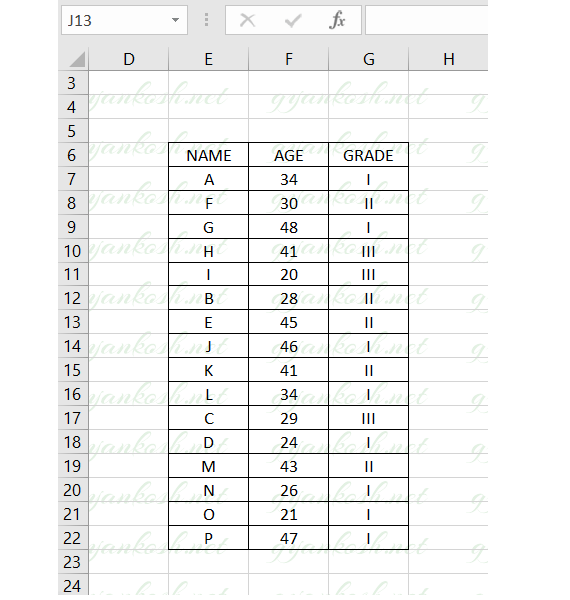
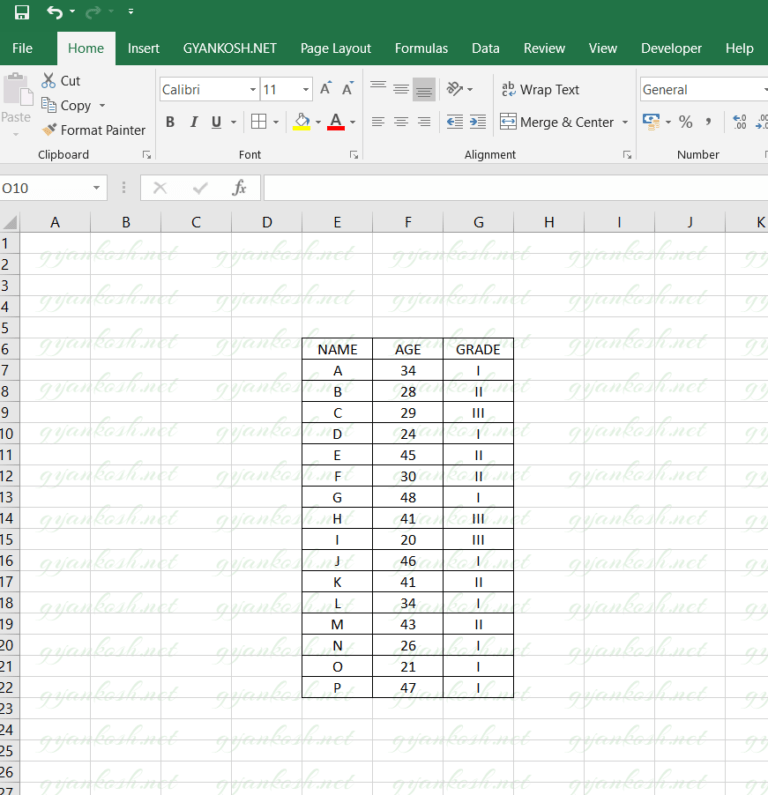
The following picture shows a table of different people showing their age and the grade.
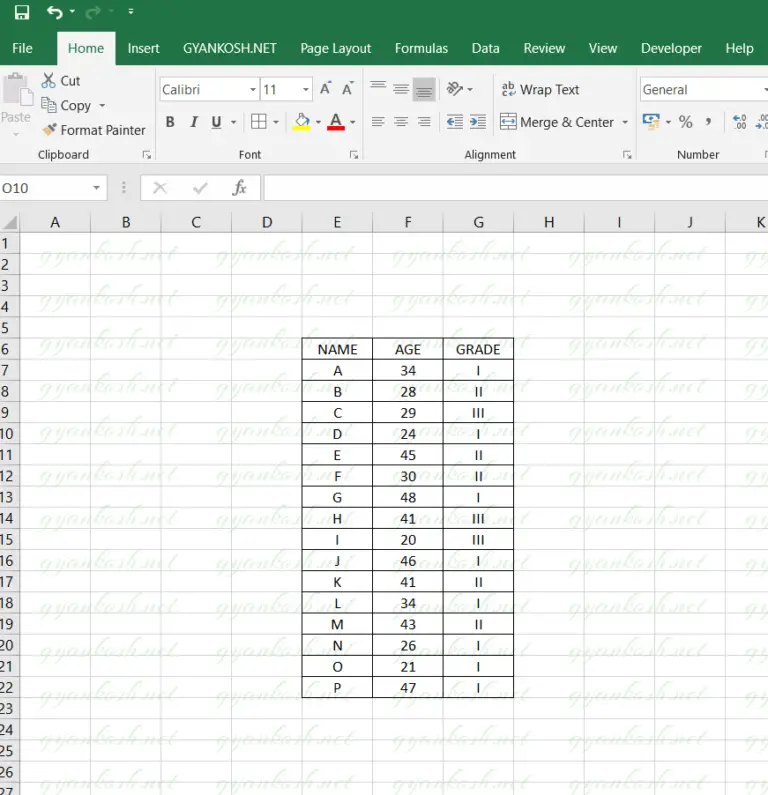
The following picture shows the original data.

We have sorted the data with respect to the NAME COLUMN.
We again sorted it with respect to the AGE COLUMN and again with respect to the NAME COLUMN. It means we performed the sorting operation thrice.
After sorting the table, the data looks like the one shown in the picture below.
Now, we can reverse it step by step using the UNDO BUTTON operation or by pressing CTRL+Z or we can use the direct method.
For the direct method we need to press a small DOWNWARD BUTTON with the UNDO BUTTON.

After clicking the dropdown button, we’ll see the list of complete actions performed on our data.
NOTE: BY DEFAULT EXCEL WILL STORE UPTO 100 ACTIONS PERFORMED.
The following picture shows the list of steps.
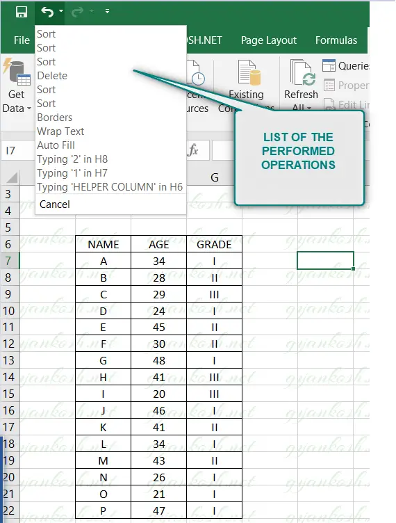
We can notice the THREE SORT OPERATIONS AT THE TOP which are performed by us and we intend to reverse them.c
So, move the mouse to the third SORT OPERATION from the top. [ Which is actually the first operation as the last operation will be placed at the top just like a STACK ].
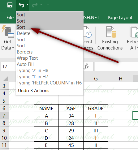
Click the third sort operation from the top.
The three sort operations will be reverted and we’ll get our original data after the reversal of the SORT OPERATION AS SHOWN IN THE PICTURE BELOW.
UNSORT DATA IN EXCEL USING HELPER COLUMN
This method is foolproof but needs to be used before we start any kind of SORTING OPERATION on our data.
Let us take a sample data to learn the process.
The data is same as used for the previous method.
The following picture shows the Names of the employees with age as well as grade placed randomly.
The data shown above is the original sequence of the data.
If we want to preserve it, or if we doubt that a situation may occur when we need to recover this data or bring the original data, follow the steps.
STEPS TO UNSORT THE DATA.
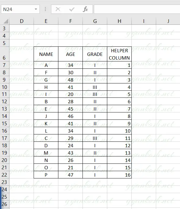
- Before, sorting the data, create a helper column and name it as per you wish . For our example we’d call it HELPER COLUMN as shown in the picture below.
- Put the content in the column as the location number starting from 1 up to the last number. For this, simply type 1 , 2 … in a few rows and then drag down the formula through the last row of the data.
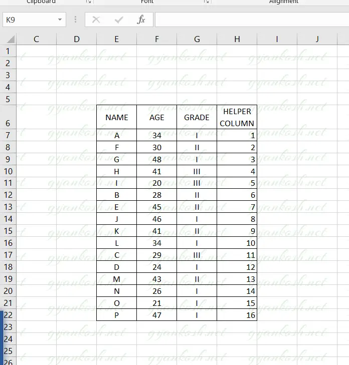
- In the mentioned example, we have 16 items so in our helper column the number goes from 1 to 16. This is the actual initial position of the items.
- Now we are free to sort the items as the way we want. We are free to do any operation [Except the operation which create any change in the helper column data].
For the completion of our example, let us perform some random operations on our data.
YOU CAN LEARN SORTING IN EXCEL HERE.
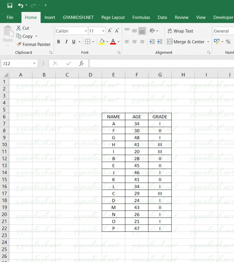
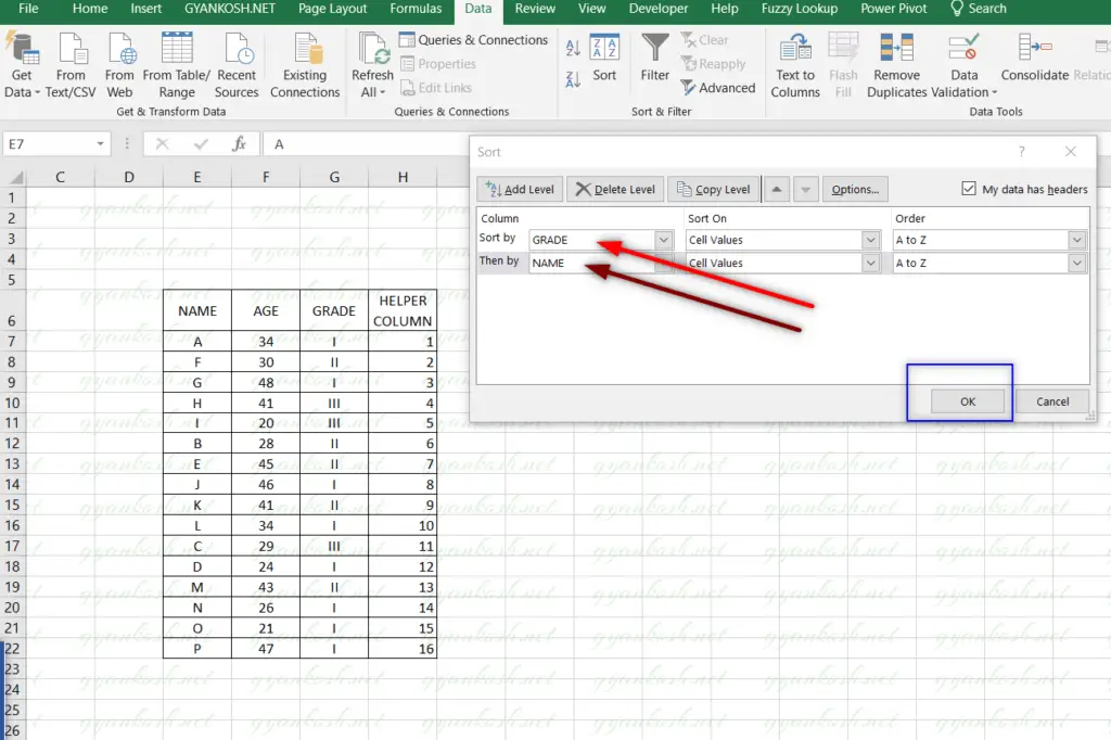
We performed a few sorting operations and sorted the data [MULTILEVEL SORT ] with respect to GRADE and NAME columns.
After the sorting, our data will be something like this.
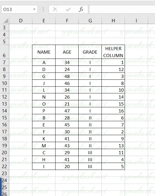
In the above picture, we have performed random operations on the data.
After the sorting, the data looks like the one shown in the picture below.
TO UNSORT THE DATA
Simply sort the data in the ASCENDING ORDER by the helper column.
It’ll bring back the original sequence of the items as required.
Follow the steps to sort the data as per helper column.
- Select the Table.
- Go to DATA TAB > SORT . [ FOR IN-DEPTH DETAILS CLICK HERE ]
- The SORT DIALOG BOX will open.
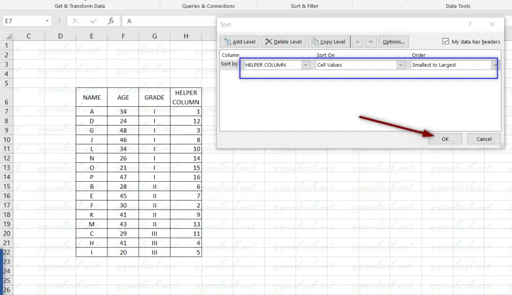
- Choose COLUMN SORT BY as HELPER COLUMN, SORT ON as CELL VALUES and Order as SMALLEST TO LARGEST as shown in the picture below.
- Click OK.
- After clicking the sort, the data will be sorted as per the HELPER COLUMN and the process will remove all the sorting or any other steps which changed the order of the data.
- The picture below shows the original data after the reversal of the sorting.
We can remove the HELPER COLUMN if we don’t need it further.
NOTE: IF YOU THINK THAT THE ORIGINAL DATA MIGHT BE NEEDED IN FUTURE, YOU SHOULD ALWAYS KEEP A COPY OF THE DATA OR KEEP YOUR HELPER COLUMN INTACT.