Table of Contents
- INTRODUCTION
- HOW DATE IS HANDLED IN EXCEL?
- WHAT IS CONDITIONAL FORMATTING BASED ON DATES?
- EXAMPLES SHOWING CONDITIONAL FORMATTING BASED ON DATES
- EXAMPLE 1: HIGHLIGHT ALL THE DATES PRIOR TO A GIVEN DATE
- EXAMPLE 2: HIGHLIGHT ALL THE DATES LATER THAN A GIVEN DATE
- EXAMPLE 3: HOW TO HIGHLIGHT THE DUPLICATE DATES IN THE GIVEN CELLS IN EXCEL SHEET?
- EXAMPLE 4: HOW TO HIGHLIGHT TODAY’S DATE USING CONDITIONAL FORMATTING IN EXCEL?
- EXAMPLE 5: HOW TO HIGHLIGHT DATES OLDER THAN THIRTY DAYS [30] USING CONDITIONAL FORMATTING IN EXCEL?
- EXAMPLE 6: HOW TO HIGHLIGHT DATES WITHIN THIRTY DAYS [30] USING CONDITIONAL FORMATTING IN EXCEL?
- FAQs
- HOW TO HIGHLIGHT THE DATES PAST DUE DATE?
INTRODUCTION
Whenever we prepare any report in excel, we have two constituents in any report.
The Text portion and the Numerical portion.
But just storing the text and numbers doesn’t make the super reports. Many times we need to automate the process in the reports to minimize the effort and improve the accuracy.
Many functions are provided by Excel which works on Text and gives us useful output as well. But a few problems are still left on which we need to apply some tricks with the available tools.
THIS WAS AN EXCERPT FROM THE FIRST ARTICLE OF THIS SERIES MANIPULATING DATES IN EXCEL – PART I
We will continue learning many more techniques about the manipulation of text in Excel.
In this article, we’ll learn the way to deal with the dates in CONDITIONAL FORMATTING in Excel.
HOW DATE IS HANDLED IN EXCEL?
The first and foremost point is to understand how Excel handles the dates. What are the dates for Excel?
Date is treated as a simple serial number by excel starting from Jan 1 1900 [ treated as 1].
From Jan 1, 1900 which is 1 for Excel the serial number starts and it is still going on .
For example, it is 29th June 2020 today so the serial number for this date is 44011.
If I type this number in Excel simply,
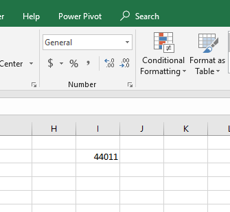
and convert the format to date, It’ll translate it to the date mentioned above which is 29-06-2020.
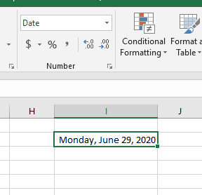
By the pictures shown above, it is clear that we can play with the dates in both ways.
We can write the date in the various DATE FORMATS or we can simply use the numbers.[ Of course, it is not easy to remember the numbers, but we can refer for once].
EXCEL HAS THE PROVISION OF DATES FROM JAN 1,1900 TO DEC 31, 9999 which corresponds to 2958465.
So it should be clear to the Excel user that the date is nothing but a number. But why the problem occurs then.
The problem occurs when we think that the given format is Date but Excel doesn’t accept it as a date. It happens when we violate the rules of entering the date when we try to enter the date from various formats mentioned below.
WHAT IS CONDITIONAL FORMATTING BASED ON DATES?
CONDITIONAL FORMATTING is the process of formatting in Excel on the basis of the conditions. We can put many conditions in the cell and program the Excel to make the formatting, as desired if the particular condition is met.
Formatting comprises of the foreground color, background color, font, size, etc. which are the properties of the text.
It makes the results more readable.
IT IS RECOMMENDED TO LEARN THE BASICS OF CONDITIONAL FORMATTING, IF NOT VERY COMFORTABLE WITH THIS TOPIC.
CLICK HERE TO LEARN ABOUT CONDITIONAL FORMATTING.
Maximum times, we apply conditional formatting on the basis of values present in the cells.
Let us now learn the way by which we can apply conditional formatting based on DATES.
EXAMPLES SHOWING CONDITIONAL FORMATTING BASED ON DATES
We’ll take different examples showing the use of conditional formatting under various circumstances.
We’ll need to find out the various situations such as the possible window for a few days, next n days, previous n days, and many other situations like that.
EXAMPLE 1: HIGHLIGHT ALL THE DATES PRIOR TO A GIVEN DATE
We can highlight all the dates which are prior to a given date very easily.
Let us highlight all the dates which are prior to 5/24/2021 out of all the given dates.
Let us take an example showing different dates as shown below.
| 5/24/2021 | 2/10/2022 | 8/16/2021 | 9/27/2021 | 7/16/2021 | 7/29/2021 | 9/29/2021 |
| 5/7/2021 | 2/8/2022 | 6/7/2021 | 1/11/2022 | 11/1/2021 | 3/31/2022 | 8/13/2021 |
| 6/2/2021 | 4/27/2021 | 6/27/2021 | 9/24/2021 | 2/12/2022 | 12/8/2021 | 2/7/2022 |
| 3/6/2022 | 4/19/2021 | 4/25/2021 | 12/8/2021 | 3/26/2022 | 7/26/2021 | 7/22/2021 |
| 8/13/2021 | 12/9/2021 | 5/8/2021 | 11/20/2021 | 5/3/2022 | 8/10/2021 | 12/20/2021 |
| 6/24/2021 | 4/18/2021 | 10/27/2021 | 5/20/2021 | 9/19/2021 | 4/15/2021 | 2/19/2022 |
| 11/16/2021 | 11/2/2021 | 3/9/2022 | 2/4/2022 | 2/1/2022 | 7/27/2021 | 3/22/2022 |
| 12/25/2021 | 1/30/2022 | 4/27/2021 | 7/16/2021 | 11/22/2021 | 2/25/2022 | 1/23/2022 |
FOLLOW THE STEPS TO HIGHLIGHT THE DATES PRIOR TO A GIVEN DATE. [ HIGHLIGHT DATES PRIOR TO 5/24/2021 ]
- We have the following example data. [ Your data may comprise of a few columns or cells or specific rows etc. ]
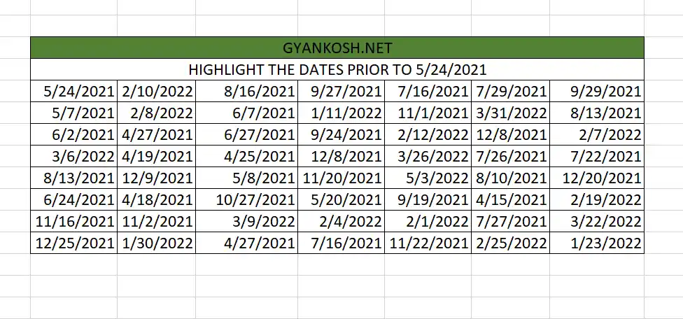
- Select all the cells containing the dates i.e. the cells on which you want to apply conditional formatting.

- Go to CONDITIONAL FORMATTING> HIGHLIGHT CELLS RULES >LESS THAN under the HOME TAB.
- The location is shown below.
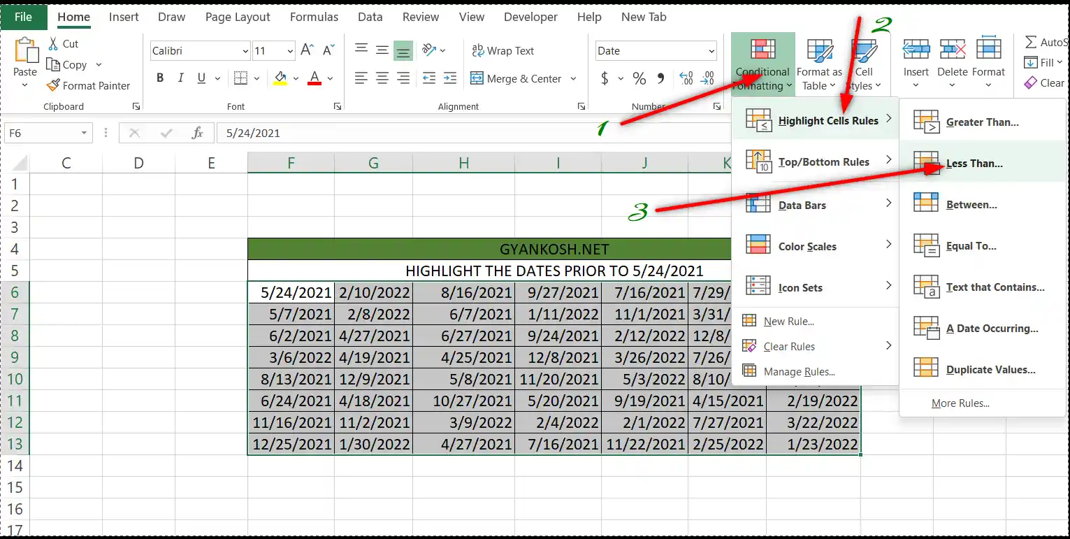
- As we choose the LESS THAN option, a small window will open.
- Enter the cut-off date as 5/24/2021 i.e. the date prior to which, you want to highlight the dates.
- Click OK.
- All the dates earlier to 5/24/2021 will be highlighted.
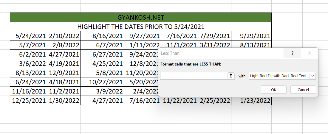
This is the way to highlight the cells earlier to any specific date.
CONCEPT:
We simply used the LESS THAN option, which is normally used to highlight the numbers because DATE is itself a number. Date is a format which is used as a mask on the number which represents a particular date. REFER HOW DATE IS HANDLED IN EXCEL for further details.
So, if we put the DATE NUMBER or the date in the LESS THAN field, it’ll highlight all the dates prior to the given date. For our example, it’ll highlight all the dates prior to 5/24/2021.
EXAMPLE 2: HIGHLIGHT ALL THE DATES LATER THAN A GIVEN DATE
So, this example is exactly opposite to the one we just discussed. [ Example 1].
The procedure is exactly the same as Example 1 except the option which we choose from the CONDITIONAL FORMATTING Menu.
Follow the steps to highlight all the dates later than a given date.
- Select all the cells on which you want to apply conditional formatting . [ The cells where you want to put the condition. ]
- Go to HOME TAB > CONDITIONAL FORMATTING >HIGHLIGHT CELL RULES > GREATER THAN.
- The window will open.
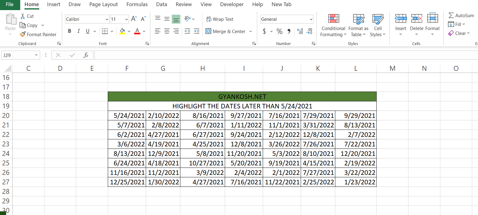
- Enter the cut off date . [ All the dates falling after the cut off date will be highlighted. ] For our example, we’ll enter 5/24/2021.
- Choose the color of your choice which will be chosen for highlighting.
- We are done.
EXAMPLE 3: HOW TO HIGHLIGHT THE DUPLICATE DATES IN THE GIVEN CELLS IN EXCEL SHEET?
Extending the same example, let us try to find out the date repetition in the given data.
DATE REPETITION is simply the occurrence of the same date more than once.
Let us try an example to learn the way which will let us highlight all the repetitive dates in the given data.
The data example is the same.
| 5/24/2021 | 2/10/2022 | 8/16/2021 | 9/27/2021 | 7/16/2021 | 7/29/2021 | 9/29/2021 |
| 5/7/2021 | 2/8/2022 | 6/7/2021 | 1/11/2022 | 11/1/2021 | 3/31/2022 | 8/13/2021 |
| 6/2/2021 | 4/27/2021 | 6/27/2021 | 9/24/2021 | 2/12/2022 | 12/8/2021 | 2/7/2022 |
| 3/6/2022 | 4/19/2021 | 4/25/2021 | 12/8/2021 | 3/26/2022 | 7/26/2021 | 7/22/2021 |
| 8/13/2021 | 12/9/2021 | 5/8/2021 | 11/20/2021 | 5/3/2022 | 8/10/2021 | 12/20/2021 |
| 6/24/2021 | 4/18/2021 | 10/27/2021 | 5/20/2021 | 9/19/2021 | 4/15/2021 | 2/19/2022 |
| 11/16/2021 | 11/2/2021 | 3/9/2022 | 2/4/2022 | 2/1/2022 | 7/27/2021 | 3/22/2022 |
| 12/25/2021 | 1/30/2022 | 4/27/2021 | 7/16/2021 | 11/22/2021 | 2/25/2022 | 1/23/2022 |
FOLLOW THE STEPS TO HIGHLIGHT ALL THE DUPLICATE DATES IN EXCEL
- Select all the cells containing dates where you want to search for the duplicate dates.
- Go to HOME TAB> CONDITIONAL FORMATTING >HIGHIGHT CELL RULES >DUPLICATE VALUES.
- As we click this option, a small window will open.
- Select the formatting and click OK.

EXAMPLE 4: HOW TO HIGHLIGHT TODAY’S DATE USING CONDITIONAL FORMATTING IN EXCEL?
It is one of the very easy tasks to do using conditional formatting.
FOLLOW THE STEPS TO HIGHLIGHT TODAY’S DATE IN EXCEL
- Select all the cells containing dates where you want to search for the duplicate dates.
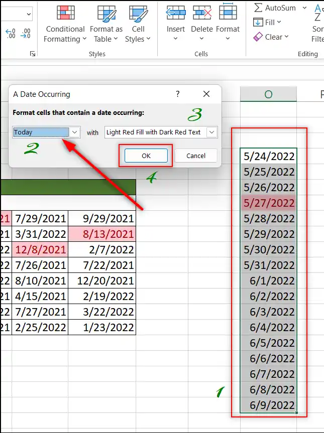
- Go to HOME TAB> CONDITIONAL FORMATTING >HIGHIGHT CELL RULES >A DATE OCCURRING.
- As we click this option, a small window will open.
- Choose TODAY from the dropdown.
- Select the format and click OK.
- If TODAY’S DATE is available, it’ll be highlighted. [ If current date i.e. today’s date is not in the list, it won’t be highlighted. ]
EXAMPLE 5: HOW TO HIGHLIGHT DATES OLDER THAN THIRTY DAYS [30] USING CONDITIONAL FORMATTING IN EXCEL?
It is one of the frequently required operations where we need to highlight the dates older than 30 days or vice versa.
Let us highlight the dates older than thirty days from the current date.
FOLLOW THE STEPS TO HIGHLIGHT THE DATES OLDER THAN 30 DAYS.
- Select all the cells containing dates where you want to search for the duplicate dates.
- Go to HOME TAB> CONDITIONAL FORMATTING >NEW RULE.
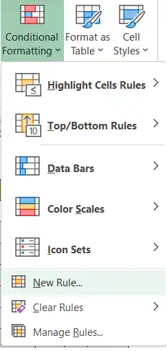
- As we click this option, a window will open.
- Choose the last RULE TYPE as USE A FORMULA TO DETERMINE WHICH CELLS TO FORMAT.
- A field to enter the formula will open.
- Enter the formula as F62<(TODAY()-30) where F62 is the first cell of the selection. [ If your cell is A1, it’ll be A1 , if B6 then it’ll be B6 ].
- Click FORMAT BUTTON and choose the format which you want to set for the cells that will fulfill the condition. [ FOR DETAILED LEARNING CLICK HOW TO USE CONDITIONAL FORMATTING IN EXCEL?
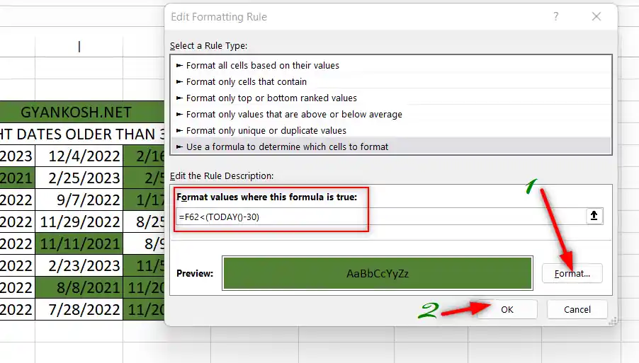
- After selecting the format, click OK.
- The result will highlight all the dates which are older than 30 days.

This was the way to highlight the dates older than 30 days in Excel using conditional formatting.
EXAMPLE 6: HOW TO HIGHLIGHT DATES WITHIN THIRTY DAYS [30] USING CONDITIONAL FORMATTING IN EXCEL?
Let us now highlight the dates within 30 days from current date. [ It is 5/28/2022 today for the example ]
FOLLOW THE STEPS TO HIGHLIGHT THE DATES WITHIN 30 DAYS
- Select all the cells containing dates where you want to search for the duplicate dates.
- Go to HOME TAB> CONDITIONAL FORMATTING >NEW RULE.

- As we click this option, a window will open.
- Choose the last RULE TYPE as USE A FORMULA TO DETERMINE WHICH CELLS TO FORMAT.
- A field to enter the formula will open.
- Enter the formula as F62>(TODAY()-30) where F62 is the first cell of the selection. [ If your cell is A1, it’ll be A1 , if B6 then it’ll be B6 ].
- Click FORMAT BUTTON and choose the format which you want to set for the cells that will fulfill the condition. [ FOR DETAILED LEARNING CLICK HOW TO USE CONDITIONAL FORMATTING IN EXCEL?
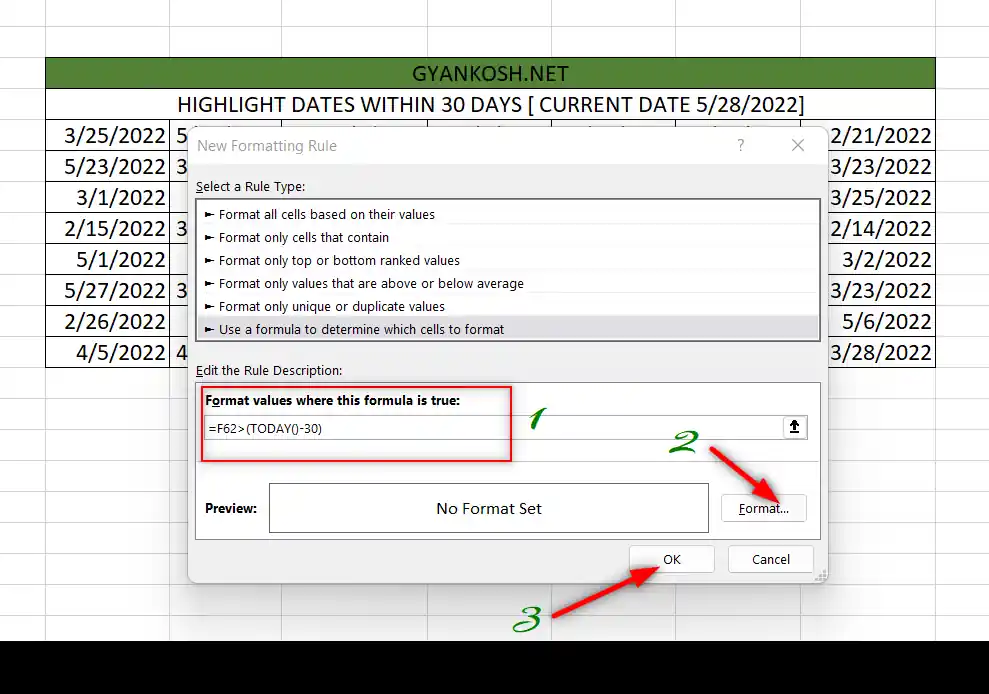
- After selecting the format, click OK.
- The result will highlight all the dates which are older than 30 days.
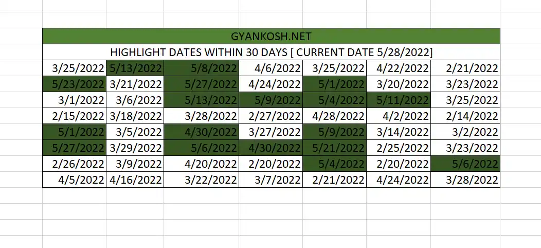
This was the way to highlight the dates within 30 days in Excel using conditional formatting.
FAQs
HOW TO HIGHLIGHT THE DATES PAST DUE DATE?
This is again one of the frequent requirement in Excel. Let us try to solve this.
We can simply use the EXAMPLE 2 WAY for the reference.
Simply put the DUE DATE as the cut off date after going to CONDITIONAL FORMATTING>GREATER THAN.
All the dates past the due date will be highlighted.