Table of Contents
- INTRODUCTION
- DIFFERENT WAY TO TROUBLESHOOT FORMULAS IN EXCEL
- WHERE DO WE FIND TRACE PRECEDENTS, TRACE DEPENDENTS, SHOW FORMULAS, EVALUATE FORMULA OPTIONS IN EXCEL
- STEPS TO TROUBLESHOOT IN EXCEL
- HOW TO MAKE THE FORMULAS APPEAR IN EXCEL?
INTRODUCTION
Excel is a great analytical tool which gives us countless options to create charts, automated reports and so many amazing tasks.
We make big reports in Excel which comprise of Text, numbers , formulas, functions and more in different columns.
A small report with fewer rows and columns can be managed easily, but what if you have got a large number of columns.
Sometimes when using the complex formula we might do some mistakes which will bring out wrong results.
To avoid such conditions or if such condition is present, to rectify the issue, we need to troubleshoot the formula.
For such cases, there are few functions present in EXCEL which will help in troubleshooting these cases.
In this article, we’ll learn such tools which will help us to troubleshoot the formulas used, if they are producing wrong results.
DIFFERENT WAY TO TROUBLESHOOT FORMULAS IN EXCEL
There are different dedicated ways to troubleshoot in Excel.
Some of the ways are:
- MAKING THE FORMULAS APPEAR
- USING TRACE PRECEDENTS
- USING TRACE DEPENDENTS
- USING ERROR CHECK
- EVALUATING THE FORMULA
WHERE DO WE FIND TRACE PRECEDENTS, TRACE DEPENDENTS, SHOW FORMULAS, EVALUATE FORMULA OPTIONS IN EXCEL
We find the different troubleshooting tools such as TRACE PRECEDENTS, TRACE DEPENDENTS, SHOW FORMULAS , EVALUATE FORMULAS, ERROR CHECKING etc. under the FORMULAS TAB. [ RIGHT PORTION] .
The location is shown in the picture below.
STEPS TO TROUBLESHOOT IN EXCEL
Troubleshooting needs to scan your data a number of ways to find out the culprit which is causing the wrong result.
First of all , let us try to check the formulas and see if we are using the correct references.
HOW TO MAKE THE FORMULAS APPEAR IN EXCEL?
This is going to be the first check in our troubleshooting process.
We need to check if the formulas we are using have the correct references or not.
It means, if we want to add column A to the column C , check if we are not using any other column in place or A or C.
For checking the formulas we can go either of the two ways
- Select every cell and check for the formulas. or
- Press CTRL+` or go to FORMULAS TAB and press SHOW FORMULAS which will make all the cells containing the calculations to show the formulas in place of results.
Now, it is obvious that it is easier to check the formulas if they are already visible which makes the WAY NO. 2 better than number 1.
STEPS TO SHOW USED FORMULAS IN EXCEL
- Simply press CTRL+`.
- Alternatively, go to FORMULAS TAB and check SHOW FORMULAS.
All the formulas will become visible.
Check all the formulas if you have used the correct references or not.
HOW TO HIDE THE FOMULAS IN EXCEL ?
- After you are done, use the same process again to hide the formulas, as it is a toggle function.
- Press CTRL+` or go to FORMULAS TAB and uncheck SHOW FORMULAS again to hide all the functions used.
If you couldn’t find the error yet, try the next way.
HOW TO USE TRACE PRECEDENTS IN EXCEL ?
The one way to search for any mess is by checking the cells which are sending the values to the current cell [ which is under inspection.]
For this, we have a dedicated option known as TRACE PRECEDENTS.
TRACE PRECEDENTS helps us to trace the cells which are dependent on the current selected cell. This options shows all the cells which are involved in the derivation of result in the current cell.
Let us try to learn the usage of TRACE PRECEDENTS using the following example.
Example-
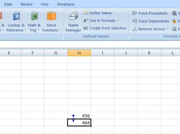
Suppose we added 8 to a value in a cell. Now keep the cursor in result and click TRACE PRECEDENTS.
We added 8 to 456.
So the result shows that the value has derived by acting upon the CELL SHOWN.
AN ARROW SHOWS THE PROCESS OF THE FLOW. FOR THE DISCUSSED EXAMPLE, AN ARROW STARTS FROM THE CELL CONTAINING THE VALUE 456 AND ENDS UP IN THE CELL WHICH WE SELECTED TO CHECK THE PRECEDENTS.
So, in this way we can find out the precedents for any cell in Excel.
If, this doesn’t help us, we’ll further go to next tool known as TRACE DEPENDENTS.
Now, there can be a requirement when we want to search out the cells which are dependent on the current cells.
HOW TO USE TRACE DEPENDENTS IN EXCEL?
TRACE DEPENDENTS is another very powerful tool to search out the relationship between the cells.
TRACE DEPENDENTS shows all the cells which contain the values, whose values are dependent on the selected cell value or simply stating, it’ll show all the CELLS which contain any formula referring to the selected cell.
EXAMPLE:
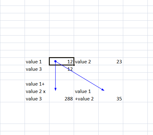
Suppose we select a cell and use it in two different formulas. Now select the first cell and click TRACE DEPENDENTS.
Two arrows will appear as shown in the picture below.
The picture will make it more clear.
This picture shows that the VALUE 1 has been used in two cells which are pointed by the arrows.
Even if we couldn’t search out the error, we ‘ll use the next way. But before that , we need to remove the arrows which appeared by the use of TRACE DEPENDENTS AND TRACE PRECEDENTS. Follow the next section.
HOW TO REMOVE ARROWS WHICH APPEARED BY USING TRACE DEPENDENTS AND TRACE PRECEDENTS?:
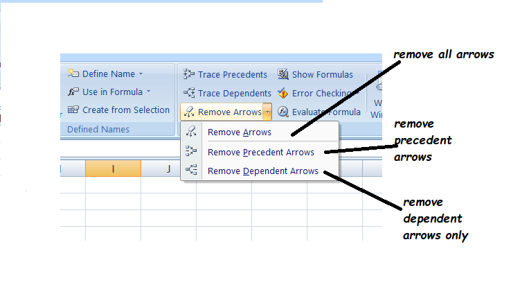
Simply go to the FORMULA TAB and choose the appropriate option from the dropdown.
The options and their effect has been shown in the picture below.
It removes the arrows which appeared in the trace dependents and trace precedents as per the picture.
Next option is to use the ERROR CHECKING option.
HOW TO USE ERROR CHECKING ?
Have you ever encountered a situation where EXCEL itself tells that your formula has an error.
This option will help you out if that is the case.
This option gives the facility of checking any error. Select the error cell and click ERROR CHECKING. The dialog will show help on the error which can be rectified.
For Example,
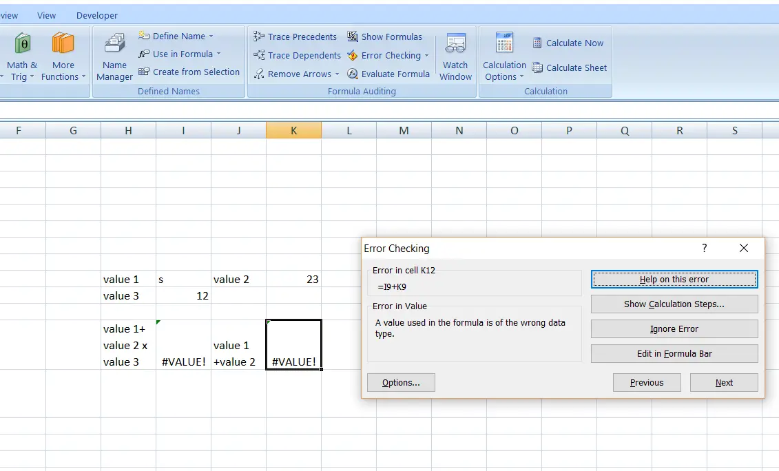
We created a problem in a cell by putting a text in a cell whose value was used in the result. Selected the cell and clicked ERROR CHECKING.
The screen shows its observation.
As we selected the cell and clicked on ERROR CHECKING, it simply gave us the information about the same.
You can check in the picture above, that the section ERROR IN VALUE is showing the reason A VALUE USED IN THE FORMULA IS OF THE WRONG DATA TYPE.
Such help can prove to be of immense help sometimes.
One more tool is present especially for the step wise step evaluation of the formula used known as Evaluate Formula.
HOW TO CHECK STEP WISE STEP VALUES IN FORMULAS USING EVALUATE FORMULA OPTION IN EXCEL?
This is one of the very useful tool provided in Excel.
It shows the steps of the evaluation. Many times especially in complex formulas, it might happen that the result is not as per our expectations and we are not able to find out the issue with the formula used.
In that case this option is helpful.
EVALUATE FORMULA WILL HELP US TO CHECK THE VALUES GIVEN TO THE DIFFERENT VARIABLES USED IN THE FORMULA STEP WISE STEP.
EXAMPLE:
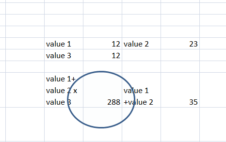
Let us take an example where we have used a formula in the encircled cell shown in the picture below.
We’ll use evaluate formula option for the same.
Lets figure out the evaluation steps of the following result.
STEPS TO EVALUATE FORMULA:
- SELECT the result cell.
- Click EVALUATE FORMULA.
- The dialog box will open and show the formula.
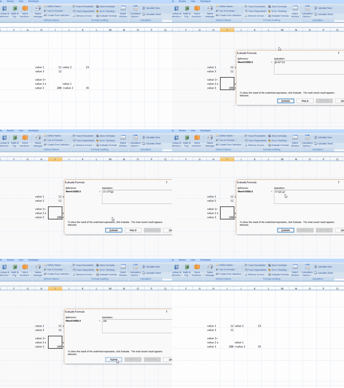
- Click EVALUATE and the formula will be replaced by values one by one. Click evaluate again and the whole process of evaluation will be shown. The process of the case discussed is shown in the following animation.
The picture above shows the working of EVALUATE FORMULA option in Excel.
One last tool , available for keeping a watch on the values is WATCH WINDOW.
HOW TO USE WATCH WINDOW IN EXCEL?
THE WATCH WINDOW:
Its a watch we keep on few cells. We can add a watch on the values.
A WATCH WINDOW HELPS US TO KEEP A WATCH OVER FEW IMPORTANT CELLS. IT OPENS UP IN A WINDOW AND IS ALWAYS VISIBLE.
It is meant for long spread data which is not visible at all the times. We keep watch on those cells whose value is to be checked again and again and we don’t want to scroll the window which will be wasting our time.
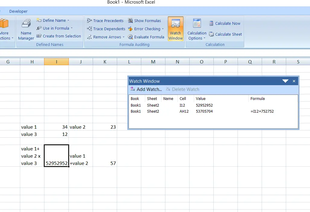
The picture shows the scenario.
In this example, AH12 cell is not visible in the window shown.
The value of AH12 is depends upon the value of I12.
So the watch will always be visible even if the window portion of AH12 is not visible.
This is the use of Watch Window for troubleshooting purpose.
HOW TO STOP OR ENABLE AUTO CALCULATION IN EXCEL:
This might be a new piece of knowledge for you.
When you change any value in a cell, the result will be changed automatically. But we have the option to stop the auto calculation.
You can find the AUTO / MANUAL CALCULATION OPTION under the CALCULATION TAB.
In manual calculation, the selected formula will be calculated only after the button CALCULATE NOW will be pressed. CALCULATE SHEET will calculate all the formulas.
In AUTOMATIC mode all the calculation will happen instantly as by default is done in EXCEL.
EXAMPLE:
Let us take two values and sum them up.
we’ll disable the auto calculation and change the values of one of the two values and see if the auto calculation stops or not.
STEPS FOR CALCULATION OPTION:
- SELECT the result cell.
- Go to FORMULA TAB and search for the CALCULATION SECTION on the RIGHT of the RIBBON.
- Click CALCULATION OPTIONS DROPDOWN and choose MANUAL.
- The auto calculation will be stopped.
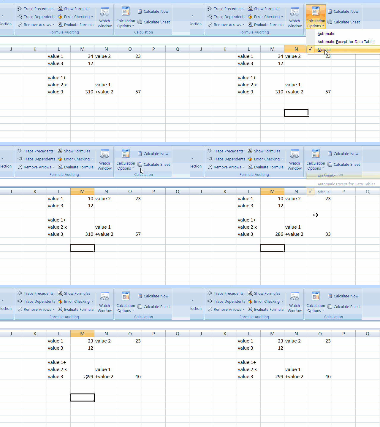
- The following picture shows the process.
It is clearly shown that when we choose the CALCULATION to be MANUAL, there is no change in the result even when we changed the values. But otherwise, when the calculation is AUTO, it changes immediately.
There can be rare situations when we need such condition that we want the result only after all the editing is done.
This option is perfect for that situation.

