Table of Contents
- INTRODUCTION
- WHERE DO WE FIND BUTTON LOCATION TO FREEZE PANES IN EXCEL ?
- WHAT IS FREEZING ROWS/ COLUMNS /PANES IN EXCEL?
- WHAT IS THE USE OF FREEZING ROWS OR COLUMNS?
- HOW TO FREEZE PANES IN EXCEL ?
- HOW TO UNFREEZE PANES IN EXCEL ?
- HOW TO FREEZE TOP ROW IN EXCEL?
- HOW TO FREEZE FIRST COLUMN IN EXCEL?
- ANIMATED EXAMPLE OF DIFFERENT FREEZE PANES OPTIONS IN EXCEL
- HOW TO FREEZE TOP ROW AND FIRST COLUMN SIMULTANEOUSLY ?
INTRODUCTION
Freezing panes (Certain Rows/Columns having headings etc.) in Excel is very important when we are working with big and lengthy reports .
In very large reports having many columns or rows, it becomes difficult to remember the column names and we are confused which is very irritating.
We need to scroll up the report over and again to remind us of the column or row headings.
It happens at the time of creating reports as well as when we are checking or reviewing them.
When the reports are sent to somebody, this problem emerges again.
So , our topic, freezing panes give us the solution to this very problem.
Even if we are creating the reports or we are studying them, it is always needed to know about the column or row headings otherwise it would be difficult in that case, freezing panes is very helpful as it fixes our Rows Headings or Column Headings sticking to our screen while the data can scroll up or down or left or right .
WHERE DO WE FIND BUTTON LOCATION TO FREEZE PANES IN EXCEL ?
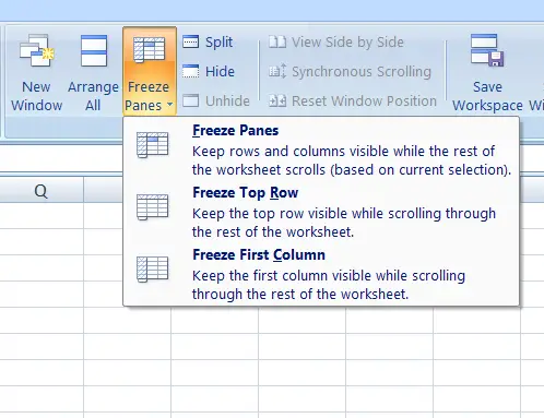
FREEZE PANES options are found under VIEW tab in WINDOW subsection as shown in the picture below.
WHAT IS FREEZING ROWS/ COLUMNS /PANES IN EXCEL?
FREEZING ROWS/ COLUMNS / PANES means to freeze the top row, or top rows, or left column or left columns.
Freezing means that frozen rows or columns won’t move when we scroll the sheet left/right or up/down.
WHAT IS THE USE OF FREEZING ROWS OR COLUMNS?
FREEZING ROWS or COLUMNS is helpful to manage big reports which spread over many rows and columns.
Imagine a scenario, you are entering some data in a big report.
If you reach the rows like 100 or so , would you be able to remember the columns Headers?
No, we won’t be able to get what data is to be entered where. But if we freeze the top row containing the HEADERS, we can freeze them and it’ll make our task so much easier as the headings will be visible all the time.
HOW TO FREEZE PANES IN EXCEL ?
After we have understood the meaning and need of freezing the panes, [ Rows or Columns ], let us learn to freeze panes in Excel.
FOLLOW THE STEPS TO FREEZE ANY NUMBER OF ROWS OR COLUMNS [ PANES ]
- Select the cell where you want to freeze the rows or columns or both.
- Click FREEZE PANES.
The rows above the selected cell and column left to the selected cell will be frozen. When scrolled, rows and columns other than frozen will move.
HOW TO UNFREEZE PANES IN EXCEL ?
You can unfreeze all the columns or rows in a single go.
FOLLOW THE STEPS TO UNFREEZE ALL THE ROWS OR COLUMNS IN EXCEL
- Go to VIEW TAB and click UNFREEZE PANES.
- No need to select any row or column. Just click unfreeze panes and it’ll unfreeze any frozen pane.
The following picture shows the button location.
The demonstration is given in the animated picture below.

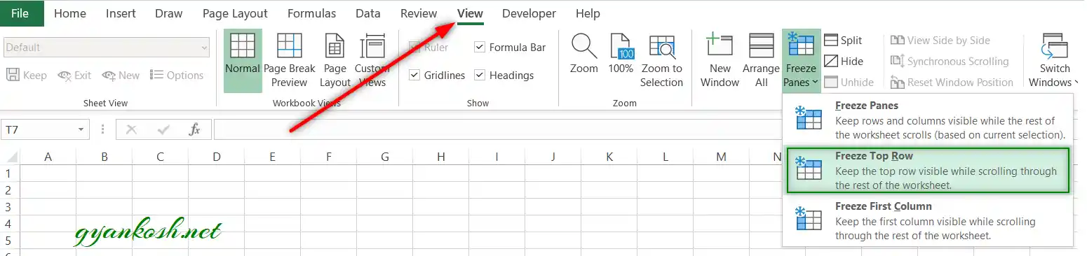
HOW TO FREEZE TOP ROW IN EXCEL?
We can freeze top row in excel very easily.
SIMPLY GO TO THE VIEW TAB AND CHOOSE FREEZE TOP ROW UNDER FREEZE PANES DROPDOWN.
HOW TO FREEZE TOP ROW IN EXCEL USING KEYBOARD SHORTCUT?
You can use ALT+W+F+R.
You can type this sequentially and it’ll freeze the top row.
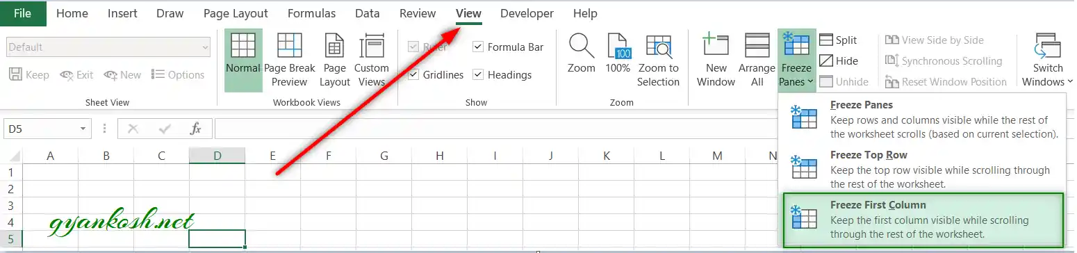
HOW TO FREEZE FIRST COLUMN IN EXCEL?
We can freeze first column in excel very easily.
SIMPLY GO TO THE VIEW TAB AND CHOOSE FREEZE TOP COLUMN UNDER FREEZE PANES DROPDOWN.
HOW TO FREEZE FIRST COLUMN IN EXCEL USING KEYBOARD SHORTCUT?
You can use ALT+W+F+C.
You can type this sequentially and it’ll freeze the top row.
ANIMATED EXAMPLE OF DIFFERENT FREEZE PANES OPTIONS IN EXCEL
EXPLANATION:
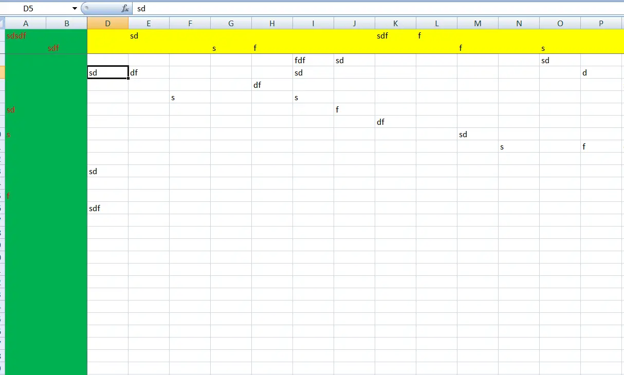
The animation starts with the demonstration of FREEZING PANES. We selected a cell, and pressed FREEZE PANES.
The rows above the cell and column left to the cell froze.
After that We used the option of FREEZING TOP ROWS, WHICH FROZE THE TOP ROW OF THE DATA. FREEZE FIRST COLUMN follows it. It freezes the first column of the sheet. After every option UNFREEZE PANES is used.
HOW TO FREEZE TOP ROW AND FIRST COLUMN SIMULTANEOUSLY ?
By using the default options to freeze top row or first column, you’ll be able to use only one of the function at a time.
To freeze top row and first column simultaneously, follow the steps.
- Select the cell B2.
- Go to VIEW TAB> WINDOWS SECTION.
- Click FREEZE PANES drop down and choose FREEZE PANES.
- The first row and first column will be frozen and won’t move.