Table of Contents
- INTRODUCTION
- BUTTON LOCATION FOR CONSOLIDATION OF DATA IN EXCEL
- TYPES OF CONSOLIDATIONS IN EXCEL
- CONSOLIDATE BY POSITION IN EXCEL
- STEPS FOR CONSOLIDATION BY POSITION IN EXCEL
- HOW TO CONSOLIDATE BY CATEGORY IN EXCEL?
- STEPS FOR CONSOLIDATION BY CATEGORY IN EXCEL
- CONSOLIDATE BY FORMULA IN EXCEL
INTRODUCTION
Consolidate, as the word itself is self explanatory helps us to mix different data by Adding, subtracting, averaging etc. kind of operations to large data in seconds and convert it into one final report or data.
It is used to consolidate scattered data into one final master file. Suppose there are many plants manufacturing chocolates everyday. Now at the headquarters, if we want to make a final statement i.e. consolidated statement, this feature can help us in a number of ways to create the data within a very short time.
BUTTON LOCATION FOR CONSOLIDATION OF DATA IN EXCEL
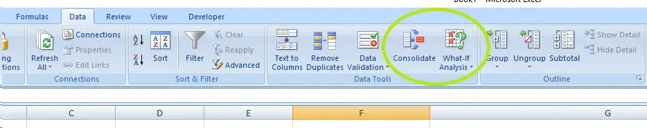
The consolidate option button can be found under the DATA TAB under DATA TOOLS SECTION.
TYPES OF CONSOLIDATIONS IN EXCEL
Consolidations can be done in the following ways.
1 CONSOLIDATE BY POSITION
2 CONSOLIDATE BY CATEGORY
3 CONSOLIDATE BY FORMULA
CONSOLIDATE BY POSITION IN EXCEL
Consolidate by position is the simplest way of consolidation process in Excel.
PREREQUISITES:
But there are many prerequisites for this process.
All the reports must have exactly same format. Same sequence of columns, rows etc.
There should not be presence of any blank or empty rows or columns.
If there is any mismatch in the columns, the result will be wrong.
STEPS FOR CONSOLIDATION BY POSITION IN EXCEL
Let us understand the steps using an example.
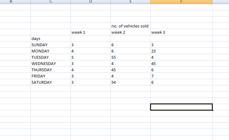
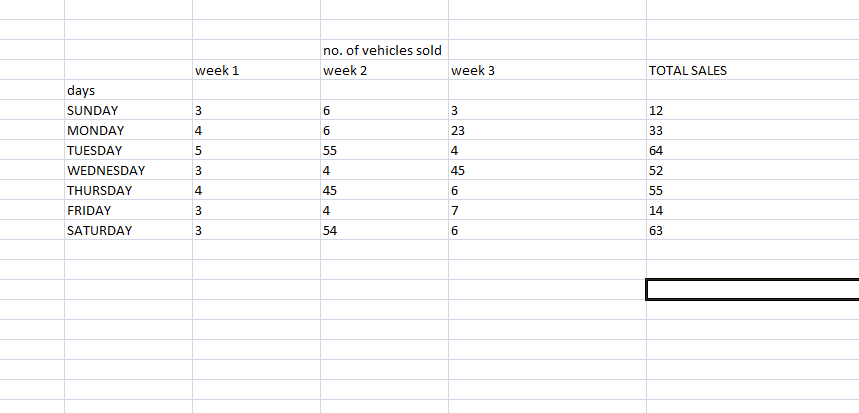
DATA Sample:
The sample shows the number of vehicle sold on different days in the three week.
select the data range and RIGHT CLICK and choose NAME A RANGE. Put the name of the range as per choice which is easy to manage.
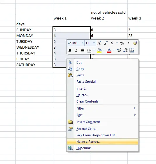
- Name all the three week data individually for every week. We have given the name as WEEK1, WEEK2 AND WEEK3.
- Click CONSOLIDATE.
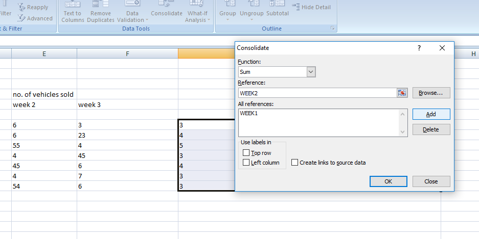
- Choose the function you want to perform. We have chosen SUM here.
- Enter the name of the first range and click ADD. The name will start appearing in ALL REFERENCES.
- Similarly enter all the names one by one and click add.
- The LABELS section will be left unchecked in this case.
- If you want to create link to source, click it, it’ll make the changes as per the change in the source data.
- CLICK OK.
- RESULT is shown in the picture below.
HOW TO CONSOLIDATE BY CATEGORY IN EXCEL?
Consolidate by CATEGORY is the MOST BENEFICIAL way of consolidation process in Excel.
PREREQUISITES:
But there are many prerequisites for this process.
THERE SHOULD NOT BE ANY REPETITION OF ANY SPELLING IN COLUMN OR ROW. Sequence can vary.
There should not be presence of any blank or empty rows or columns.
If two or more row or columns have same name, excel will result in wrong answer.
STEPS FOR CONSOLIDATION BY CATEGORY IN EXCEL
we will understand the whole process using an example.
The difference between the CONSOLIDATE BY POSITION and CONSOLIDATE BY CATEGORY is just that we can make the use of unique category names to consolidate which is very useful.
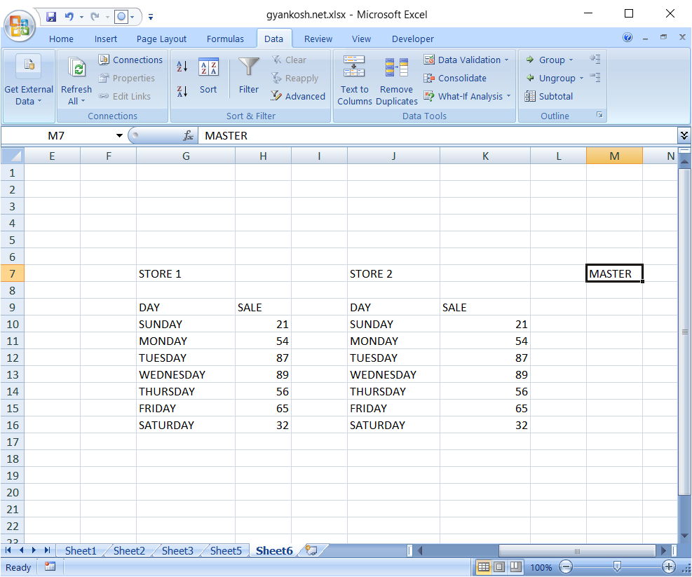
LET US TAKE A SIMILAR EXAMPLE.
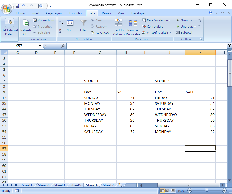
THERE ARE TWO OUTLETS WHICH ARE SELLING THE TOYS. The sales figure for a week are sent to us and we’ll make a final sheet adding the total sale of both the outlets.
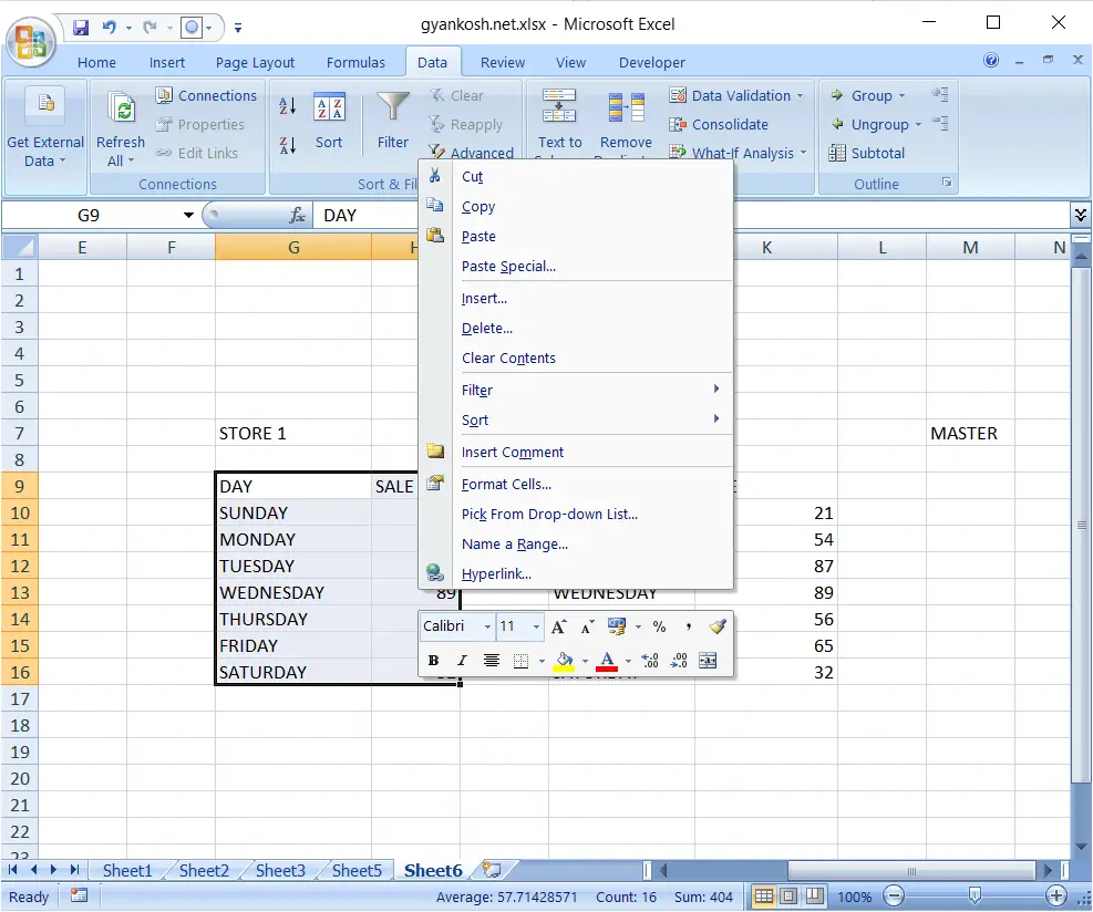
- Select the data range and RIGHT CLICK and choose NAME A RANGE. Put the name of the range as per choice which is easy to manage.
- CONSOLIDATE BY POSITION doesn’t need to include the row headings, but CONSOLIDATE BY CATEGORY needs to include the row and column names while naming a range. The process is shown in the following picture.
Select the range (NAME+VALUES) and right click and choose NAME A RANGE.
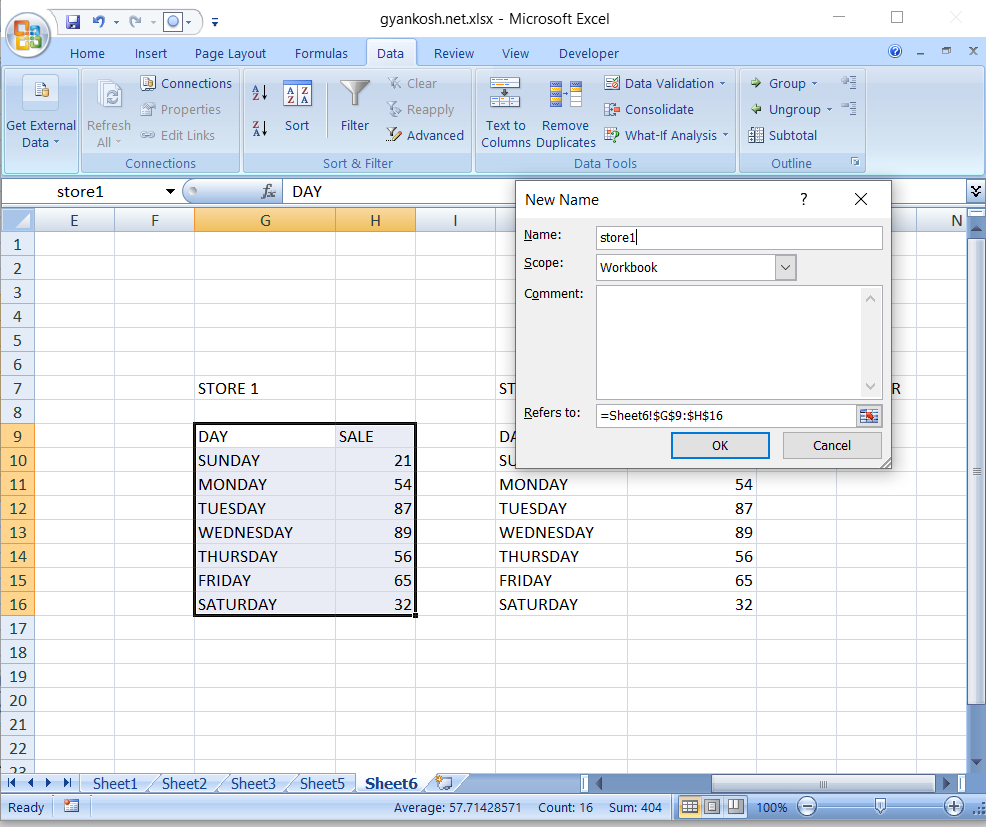
After clicking NAME A RANGE, the following dialog box will appear as shown in the picture below.In the NAME FIELD put any name which suits your need. We put store1 as name here.Choose the scope where the name can be used for. We have chosen WORKBOOK. The other option is SHEETS which can be chosen as per need if we want the name to be valid for that particular sheet only. Similarly make a range with the name STORE2 for the other store also.
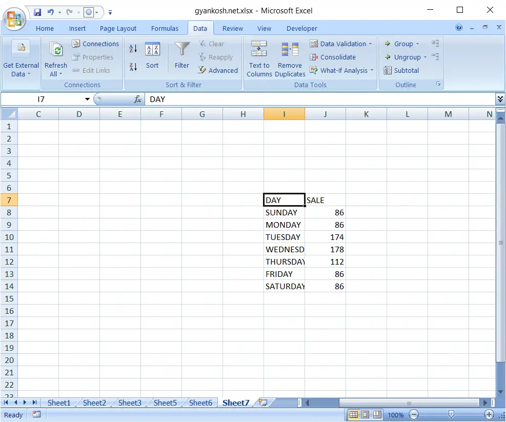
After naming both the ranges, the next step is to consolidate the data into a third table.
It is always preferable to make the consolidated table in a new sheet or other workbook.
Click a cell where you want the consolidated data to appear and click CONSOLIDATE BUTTON. The following picture will appear.
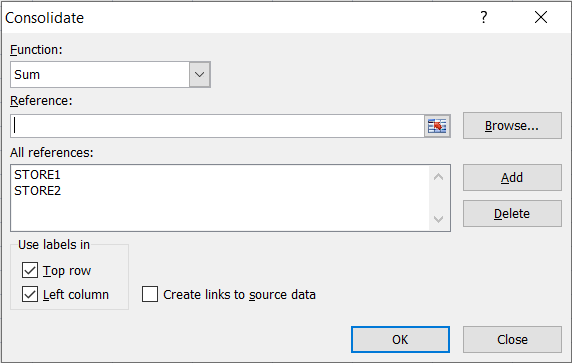
- The consolidate dialog box is shown in the picture.
STEPS:Choose the reference by selecting the cells by clicking the ICON at the right end of REFERENCE FIELD, or by typing the range, or by entering the range names as we had put STORE1 for the first one and click ADD.Again repeat the process for STORE2 and add it. Now both the names will appear in the references. Check TOP ROW or LEFT COLUMN as per need. CHECK TOP ROW, if the headings are in the top row which are to be matched, and CHECK LEFT COLUMN if the headings are in the left most column which are to be matched. Check CREATE LINKS TO SOURCE DATA if you want the data to be changed immediately if there is change in the source of the data. Click OK.
CONSOLIDATE BY FORMULA IN EXCEL
CONSOLIDATION BY FORMULA is nothing but putting a formula in the resulting cell and dragging it down to fill the rest of the column.
This is a simple way by which we make use of consolidation most of the time without even knowing that it is also a way of consolidation.
For the same example, simply put the formula for summation.
For the example as shown above , put the following formula in M10 =SUM(H10,K10) It’ll give the sum of SUNDAY SALES. after that drag the formula downwards and all the data will be filled. Again, the conditions are same as needed in the CONSOLIDATE BY POSITION. The Excel won’t come to know if the days are same or not, and totals anything present in that particular cell.