Table of Contents
- INTRODUCTION
- WHAT IS A PERCENTILE ?
- WHAT IS PERCENTRANK?
- HOW TO CALCULATE THE PERCENTRANK MANUALLY?
- WHY DO WE NEED TO CALCULATE THE PERCENTRANK IN EXCEL?
- HOW TO CALCULATE PERCENRANK IN EXCEL
- WHAT IS PERCENTRANK, PERCENTRANK.INC OR PERCENTRANK.EXC FUNCTIONS IN EXCEL?
- SYNTAX FORMULA OF PERCENTRANK FUNCTION
- EXAMPLES SHOWING THE CALCULATION OF PERCENTRANK IN EXCEL
- EXAMPLE 1:
- EXAMPLE 2: FIND OUT THE PERCENTRANK OF VALUE 76 IN THE GIVEN DATA [ AS PER EXAMPLE 1]
- FAQs
- WHAT IS THE MEANING OF PERCENTRANK IN SIMPLE WORDS?
INTRODUCTION
There are a number of accounting requirements that are not only used in any specific niche but may be required in day-to-day life.
Excel provides us with a variety of ready-to-use functions which can be used anytime to get the desired outcomes. We can also create the formulas and then get the result but it is easier to use the built-in functions that just require the input and give us the output.
One such requirement is the calculation of the PERCENTILE. [ It is not a percent which is calculated on the basis of 100 ]
Now, what if we need to calculate the reverse of percentile. Thanks to Excel, we have a ready-to-use function known as PERCENTRANK.
In percentile function, we find out the value which presents the given percentile whereas in PERCENTRANK, PERCENTRANK.INC or PERCENTRANK.EXC function we find the percentile on the basis of the given value which is in fact the rank within the given data or simply the relative standing of any value within a given data.
In this article, we’ll learn the way to calculate the percentile of any given value in Excel very easily.
WHAT IS A PERCENTILE ?
A percentile helps us to know the relative standing of the values.
A percentile is a value on a scale of 100 which will show the percent distrubution of the data set [ the values given ].
It simply means that if the highest value is 65, all the values are equal to or below it. So the 100th percentile will be 65.
Now, if we want to know the 95TH percentile, it’ll be a value, which will be higher than 95% of the total value population. [ Read this line twice for better understanding. ]
For example,
Let us take a data set of 100 values. In fact, it is a simple count from 1 to 100. [ We’ll take it as the example too later. ]
| 1 | 21 | 41 | 61 | 81 |
| 2 | 22 | 42 | 62 | 82 |
| 3 | 23 | 43 | 63 | 83 |
| 4 | 24 | 44 | 64 | 84 |
| 5 | 25 | 45 | 65 | 85 |
| 6 | 26 | 46 | 66 | 86 |
| 7 | 27 | 47 | 67 | 87 |
| 8 | 28 | 48 | 68 | 88 |
| 9 | 29 | 49 | 69 | 89 |
| 10 | 30 | 50 | 70 | 90 |
| 11 | 31 | 51 | 71 | 91 |
| 12 | 32 | 52 | 72 | 92 |
| 13 | 33 | 53 | 73 | 93 |
| 14 | 34 | 54 | 74 | 94 |
| 15 | 35 | 55 | 75 | 95 |
| 16 | 36 | 56 | 76 | 96 |
| 17 | 37 | 57 | 77 | 97 |
| 18 | 38 | 58 | 78 | 98 |
| 19 | 39 | 59 | 79 | 99 |
| 20 | 40 | 60 | 80 | 100 |
Now, the data is pretty simple.
In this data, the 95th percentile will be 95.05 as 95.05 percent values are lower or equal to 95.05.
Similarly, the 60th percentile will be 60.4 as 60% values are lower or equal to 60.4.
WHAT IS PERCENTRANK?
PERCENTRANK is the rank of any value in the given dataset as a percentage of the data set.
It simply means that it’ll show you the percentile of the value in the given dataset. This is exactly opposite to the solution given by the PERCENTILE, PERCENTILE.INC or PERCENTILE.EXC FUNCTIONS.
The PERCENTRANK will immediately give you your position among others by showing you the percentage of the people who are below you.
HOW TO CALCULATE THE PERCENTRANK MANUALLY?
PERCENTRANK can be manually calculated as
NUMBER OF VALUES LESS THAN THE VALUE OF WHICH PERCENTRANK IS TO BE FOUND / (NUMBER OF VALUES WITH VALUE MORE THAN THE VALUE OF WHICH PERCENTRANK IS TO BE FOUND + NUMBER OF VALUES LESS THAN THE VALUE OF WHICH PERCENTRANK IS TO BE FOUND )
But by using the PERCENTRANK FUNCTION in Excel, you need not to calculate anything manually, the function will do that for us.
WHY DO WE NEED TO CALCULATE THE PERCENTRANK IN EXCEL?
PERCENTRANK is a great tool to get the ranking of any value within a big dataset in a fraction of seconds.
PERCENTRANK immediately shows you the current rank within a group but the rank is shown as a percentage i.e. it’ll show the rank as a percentage within a group.
PERCENTRANK DOESN’T SHOW THE ABSOLUTE RANK.
For example, suppose a class has 100 students.
If we put them in ascending order, we can find out the absolute rank of any student.
But it won’t show the relative standing of that particular student within the class.
Say, a student Abraham got rank 10. But how would it show the relative standing in his class?
It is quite possible that there are only 10 students in the class which will make him a poor performer whereas if the total number of students is 100, the performance is not that bad. In this case, absolute rank fails to convey the proper information.
This is where PERCENTRANK comes into play.
Percentrank will show the relative standing of that student by showing the number of students whose marks are lesser than the marks secured by Abraham.
HOW TO CALCULATE PERCENRANK IN EXCEL
We can calculate the percentile of the given value easily in Excel with a ready-to-use function known as PERCENTRANK, PERCENTRANK.INC OR PERCENTRANK.EXC FUNCTION.
The PERCENTRANK FUNCTION is an older version replaced by the newer version PERCENTRANK.INC and PERCENTRANK.EXC functions. We’ll discuss the new ones.
PERCENTRANK.INC IS THE NEW VERSION OF THE OLDER PERCENRANK WHICH IS ABSOLUTELY THE SAME AS THE OLDER ONE.
WHAT IS PERCENTRANK, PERCENTRANK.INC OR PERCENTRANK.EXC FUNCTIONS IN EXCEL?
A PERCENTRANK, PERCENTRANK.INC OR PERCENTRANK.EXC , all three functions help us to find out the PERCENTRANK VALUE in EXCEL.
Percentrank function is an older function present for compatibility with the previous versions of the EXCEL.
PERCENRANK, PERCENTRANK.INC OR PERCENTRANK.EXC , ALL THREE FUNCTIONS FIND OUT THE PERCENTRANK OF ANY VALUE IN THE GIVEN DATA SET.
We’ll learn the usage with the help of a few examples given below. But before that let us learn the basics of these functions.
SYNTAX FORMULA OF PERCENTRANK FUNCTION
The syntax ( the way a function is phrased in excel) of percentrank, percentrank.inc or percentrank.exc functions in excel are given below.
PERCENTRANK FUNCTION:
=PERCENTRANK( DATA SET, VALUE FOR WHICH RANK IS TO BE FOUND, NUMBER OF SIGNIFICANT DIGITS )
DATA SET is the data that can be an array or range on which the calculations will be done.
VALUE FOR WHICH RANK IS TO BE FOUND is the value for which we’ll find out the percentrank.
SIGNIFICANT DIGITS is the number of digits after 0 i.e. decimal digits you want in your results. This argument is optional and if not used the default will be 3 digits after 0.
PERCENTRANK.INC FUNCTION:
=PERCENTRANK.INC( DATA SET, VALUE FOR WHICH RANK IS TO BE FOUND, NUMBER OF SIGNIFICANT DIGITS )
DATA SET is the data that can be an array or range on which the calculations will be done.
VALUE FOR WHICH RANK IS TO BE FOUND is the value for which we’ll find out the percentrank.
SIGNIFICANT DIGITS is the number of digits after 0 i.e. decimal digits you want in your results. This argument is optional and if not used the default will be 3 digits after 0.
PERCENTRANK.EXC FUNCTION:
=PERCENTRANK.EXC( DATA SET, VALUE FOR WHICH RANK IS TO BE FOUND, NUMBER OF SIGNIFICANT DIGITS )
DATA SET is the data that can be an array or range on which the calculations will be done.
VALUE FOR WHICH RANK IS TO BE FOUND is the value for which we’ll find out the percentrank.
SIGNIFICANT DIGITS is the number of digits after 0 i.e. decimal digits you want in your results. This argument is optional and if not used the default will be 3 digits after 0.
IT IS NOTICEABLE THAT THE ONLY DIFFERENCE IS IN THE NAME OF THE FUNCTION, THE PARAMETERS ARE THE SAME. ( The difference between both the percentrank functions .icn and .exc is discussed later in the same article.
EXAMPLES SHOWING THE CALCULATION OF PERCENTRANK IN EXCEL
EXAMPLE 1:
Let us take the same data sample as discussed earlier which contains the values from 1 to 100.
The following table shows the data table.
| 1 | 21 | 41 | 61 | 81 |
| 2 | 22 | 42 | 62 | 82 |
| 3 | 23 | 43 | 63 | 83 |
| 4 | 24 | 44 | 64 | 84 |
| 5 | 25 | 45 | 65 | 85 |
| 6 | 26 | 46 | 66 | 86 |
| 7 | 27 | 47 | 67 | 87 |
| 8 | 28 | 48 | 68 | 88 |
| 9 | 29 | 49 | 69 | 89 |
| 10 | 30 | 50 | 70 | 90 |
| 11 | 31 | 51 | 71 | 91 |
| 12 | 32 | 52 | 72 | 92 |
| 13 | 33 | 53 | 73 | 93 |
| 14 | 34 | 54 | 74 | 94 |
| 15 | 35 | 55 | 75 | 95 |
| 16 | 36 | 56 | 76 | 96 |
| 17 | 37 | 57 | 77 | 97 |
| 18 | 38 | 58 | 78 | 98 |
| 19 | 39 | 59 | 79 | 99 |
| 20 | 40 | 60 | 80 | 100 |
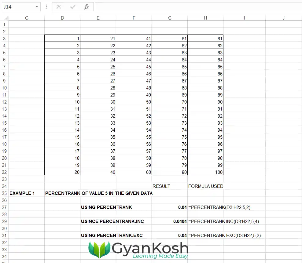
Let us find the percentrank of value 5.
FOLLOW THE STEPS TO FIND OUT THE PERCENTRANK OF 5 IN EXCEL:
- Double click the cell where you want the result.
- Enter the function as
- =PERCENTRANK( DATA RANGE, 5, 2)
- Our data resides from the cell D3 to H22 so our range becomes D3:H22.
- The formula used is
- =PERCENT.RANK(D3:H22,5,2)
- =PERCENTRANK.INC(D3:H22,5,4) [ There will be 4 digits after 0 as number of significant digits is chosen as 4 ]
- =PERCENTRANK.EXC(D3:H22,5,2)
The result appears as 0.04, 0.0404, 0.04 respectively.
0.04 MEANS THAT 0.04 [ ON A SCALE OF 1 or 4% ] OF THE VALUES ARE LESS THAN 5.
- The process is shown in the picture below.
EXAMPLE 2: FIND OUT THE PERCENTRANK OF VALUE 76 IN THE GIVEN DATA [ AS PER EXAMPLE 1]
This topic is the same as IF WE TRY TO FIND OUT THE PERCENTAGE OF VALUES WHICH ARE LESS THAN 75.
FOLLOW THE STEPS TO FIND OUT THE PERCENTRANK OF VALUE 76 IN EXCEL:
- Double click the cell where you want the result.
- Enter the function as
- =PERCENTRANK( DATA RANGE,76,2)
- Our data resides from the cell D3 to H22 so our range becomes D3:H22.
- The formula used is
- =PERCENTRANK(D3:H22,76,2)
- =PERCENTRANK.INC(D3:H22,76,4)
- =PERCENTRANK.EXC(D3:H22,76,4)
The result appears as 0.75, 0.7575, 0.7524 respectively. - The process is shown in the picture below.

So, this is the way to use the PERCENTRANK function in Excel and the ways to use PERCENTRANK, PERCENTRANK.INC OR PERCENTRANK.EXC Function in Excel.
FAQs
IS PERCENTRANK FUNCTION AVAILABLE IN EXCEL 365 or EXCEL 2019,2016,2013?
Yes. It is available but just for the sake of backward compatibility. PERCENTRANK is similar to PERCENTRANK.INC which is a newer version.
WHAT IS THE NEWER VERSION OF THE PERCENTRANK FUNCTION?
PERCENTRANK.INC function is the newer version of the older PERCENTRANK FUNCTION.
WHAT IS THE MEANING OF PERCENTRANK IN SIMPLE WORDS?
In simple words, percentrank gives the percentage of the values which are lesser than the concerned value.