UNIQUE is another new function which is still available for only OFFICE 365, Excel for Office 365 for Mac Excel for the web Excel for iPad Excel for iPhone Excel for Android tablets Excel for Android phones.
So its quite possible that you get confused and keep searching this function in your desktop version of Excel even if its 2019.
So as the name of the function appears, UNIQUE function extracts the unique values and discard the repeated values simply.
Sometimes when we are handling large reports, we come across such situations where we have large data and lot of repeated data is present. It is a cumbersome task to remove repeated data.
So this function is very easy to use and does the job perfectly. Let us see how to use this function.
PURPOSE OF UNIQUE IN EXCEL
UNIQUE FUNCTION returns a list of UNIQUE VARIABLES from the given list or range. It filters out the repeated data and keeps the unique data.
SYNTAX: UNIQUE FUNCTION
=UNIQUE(ARRAY to be operated , by rows/columns , Exactly once /All)
The UNIQUE function has the following arguments:
ARRAY to be operated It is the array which needs to be searched for unique values.
by rows/columns [optional, default-false] if true- Search for repeated rows if false-search for repeated columns
Exactly once/All [optional, default-false] if True, will result only those entry which occur only once. If false, will result those entries also which occur more than once [of course will return a single copy]
EXAMPLE 1 :UNIQUE FUNCTION
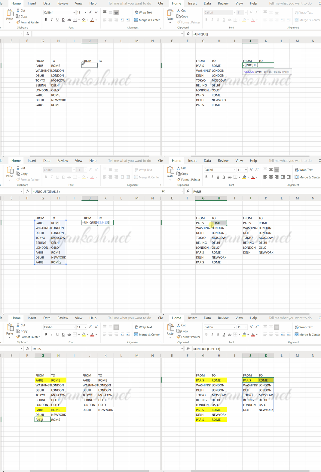
Let us try to implement the different options given in the UNIQUE FUNCTION starting with the simple usage. The data given is shown below.Its a list of flights going from one city to another.There are a few repeated entries which we would try to remove.
| FROM | TO |
| PARIS | ROME |
| WASHINGTON | LONDON |
| DELHI | LONDON |
| TOKYO | MOSCOW |
| BEIJING | DELHI |
| LONDON | OSLO |
| PARIS | ROME |
| DELHI | NEWYORK |
| PARIS | ROME |
We’ll try to remove the duplicate entries.

EXPLANATION:
We put the formula as
=UNIQUE(G5:H13)
In this example we have taken only one argument. The range G5:H13 contains all the data.
The function provides the result by keeping only one copy of repeated data as shown in the picture above.
Now let us try to see the effect of other options too.
EXAMPLE 2: REMOVE DUPLICATE COLUMNS USING UNIQUE FUNCTION
DATA SAMPLE
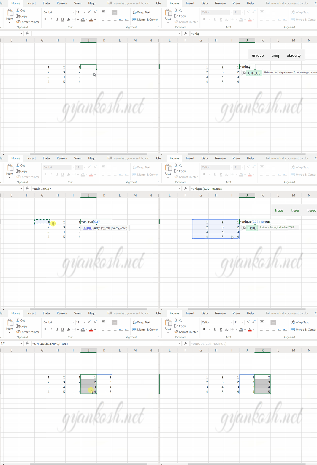
Second argument of the function decides whether the uniqueness would be found in rows or columns.Let us try this with a simple example.
| 1 | 2 | 1 |
| 2 | 3 | 2 |
| 3 | 4 | 3 |
| 4 | 5 | 4 |
Let us try to remove the duplicate columns.

EXPLANATION
The function used is
=UNIQUE(G42:I45,TRUE)
G42:I45 is the range which will be inspected for the duplicates.
True is the second argument which will make the function check the repeated columns.
We can see in the above picture that the repeated column is discarded in the results.
Let us now check the third argument.
EXAMPLE 3:INCLUDING THE ENTRIES WHICH OCCUR ONLY ONCE
DATA SAMPLE
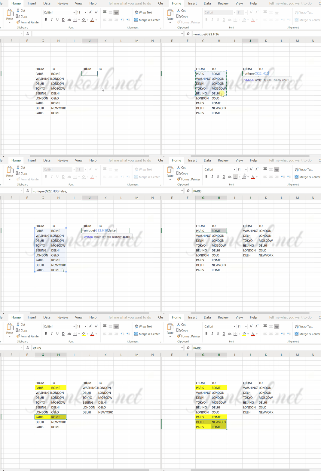
Third argument decides whether the entries with more than one copy would be kept in the result or not. Let us try this with UNIQUE function and see if it works or not.
| FROM | TO |
| PARIS | ROME |
| WASHINGTON | LONDON |
| DELHI | LONDON |
| TOKYO | MOSCOW |
| BEIJING | DELHI |
| LONDON | OSLO |
| PARIS | ROME |
| DELHI | NEWYORK |
| PARIS | ROME |
Let us try to keep only those entries which has unique single entry.

EXPLANATION
The function used is =UNIQUE(G22:H30,FALSE,TRUE)
G22:H30 is the range selected to remove the data and keep unique data.
False is kept for the row checking of duplicate entries.
The third option, which is TRUE would not let the entries which are repeated to go in the result.
We can see in the above picture that
PARIS TO ROME entry which has three entries didn’t appear in the result.
Had it been FALSE OR DEFAULT one copy of PARIS TO ROME would have been appeared.
That’s the difference.