INTRODUCTION
Case sensitive Vlookup
.If you have been working with the vlookup function of the excel for a while, you might have encountered a situation where VLOOKUP fails badly and that is, if we have the lookup value especially text with just the difference in the case of the letters i.e. Words or text with the same spelling but with different case such as BAT and bat or Bat or bAt.
There can be a number of solutions for the problem but we couldn’t find any good solution for the same.
Most of the solutions were very specific for the case such as converting all the letters to the ASCII code and then comparing, which can be done but for how many words you’d do that.
Other was to use some other function such as INDEX MATCH pair to do that. [It’ll be discussed in other post].
We decided to create a simple function which would VLOOKUP FOR A CASE SENSITIVE MATCH AND RETURN THE VALUE AGAINST THE FOUND MATCH AS PER REQUIREMENT
The article discusses the complete process of using this ADDIN [ It’s free] and get the desired result.
BENEFITS:
- No need of any lengthy formula. We have done that for you.
- Generalized solution. No custom solution needed.
FOR THE LEARNING VLOOKUP CLICK HERE.(FOR VLOOKUP IN HINDI CLICK HERE).
In this article we would learn to use VLOOKUP to extract the data from a table which has repeated or copy of lookup values differing only in the case. The function to be used is GKVLOOKUP [Gyankosh vlookup].Let us find out what it can do for us.
WHEN TO USE GKVLOOKUP
The function is very specifically meant for the situations such as:
- When you want to retrieve the value from a column which has CASE SENSITIVE INFORMATION such as two values differing only in the case. [ Easy and easy, cat and Cat and so on].
- Only the first occurrence is important. The function has the inherent problem of the Vlookup that it’ll only provide the first occurrence available from top to bottom search.
DOWNLOAD THE ADDIN
ADDIN is like a small installation to your MICROSOFT EXCEL software which adds to the capabilities of the EXCEL.
CLICK ON THE BUTTON BELOW TO DOWNLOAD THE ADDIN FOR GKVLOOKUP FUNCTION.
AFTER CLICKING THE BUTTON ABOVE, a file named gkvlookup.xlam will ask your approval to save. Save it in the desired location.
SOMETIME DUE TO SETTINGS ISSUE IF THE BROWSER TRIES TO OPEN THIS FILE AND SHOW YOU ABSURD CHARACTERS RIGHT CLICK ON THE BUTTON>SAVE LINK AS>CHOOSE LOCATION AND SAVE THE FILE.
INSTALLING THE ADDIN
ADDIN is in the form of a simple excel file with a .xlam extension.Follow the steps to install the ADDIN in Excel.
- OPEN EXCEL.
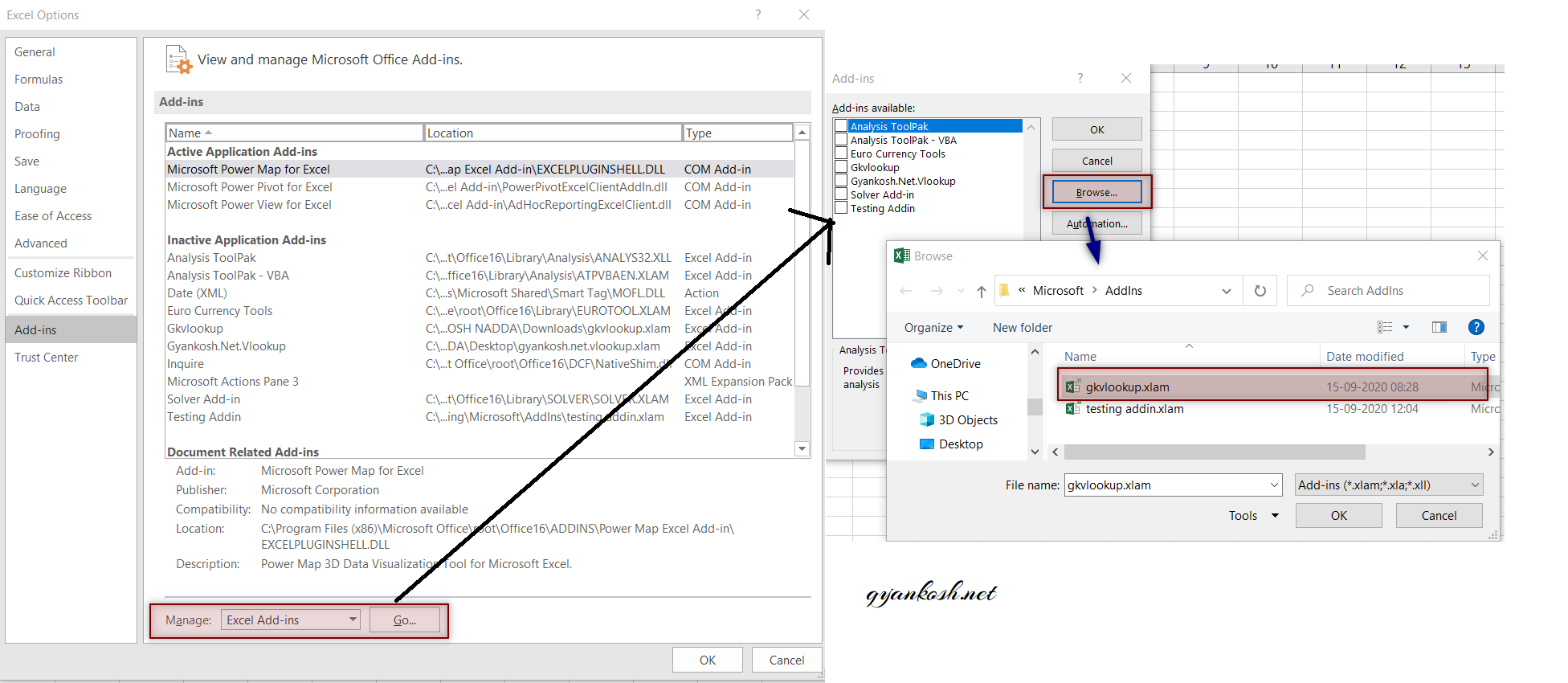
- Go to OPTIONS>ADDINS
- Select EXCEL ADD-INS
- Click GO.
- A new dialog box will open as shown in the picture containing all the EXCEL ADD-INS list.
- We can select the Addins we want to activate.
- In our case we want to install the add in , so click BROWSE.
- An OPEN FILE DIALOG BOX will open.
- Choose the file and click OK.
- The Add in will show in the list.
- Select it and click ok.
- Add in is installed.
The process is shown in the picture below.
GKVLOOKUP: SYNTAX OF FORMULA
The syntax of the GKVLOOKUP FORMULA is
=GKVLOOKUP(COMPLETE RANGE OF TABLE, VALUE TO BE MATCHED, COLUMN TO BE RETURNED )
LOOKING UP VALUES USING VLOOKUP WITH CASE SENSITIVE MATCH
FIND OUT THE VALUES AGAINST THE CODES FROM THE GIVEN TABLES.
Let us take the example of a coded language with the following codes.
We need to find out the corresponding numbers for the given codes from the given table.
| CODES | NUMBER EQUIVALENT |
| A | 1 |
| a | 1.5 |
| B | 2 |
| b | 2.5 |
| C | 3 |
| c | 3.5 |
| D | 4 |
| d | 4.5 |
| Ab | 3.5 |
| AB | 3 |
| cb | 6 |
| Cb | 5.5 |
| de | 9.5 |
From the given table, find out the code for Ab,AB,Cb,cb and c
VLOOKUP will fail in this case as it’ll always return the first instance even if the case is different but letters are same. Let us see how GKVLOOKUP performs here.
STEPS TO SOLUTION
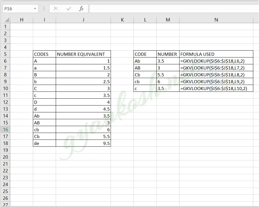
Let us find out the numbers for the given codes.
- Put the following formula in M6 (You can put the formula in any cell)
- =GKVLOOKUP($I$6:$J$18,L6,2)
- CLICK ENTER and 3.5 will appear as result.
- I6 to J18 is the table in which we’ll look up.
- 2 is the column index for the result to be returned.
- Hold the drag point in the right lower corner of the cell focus.
- Drag down the formula.
- The result will appear as shown in the picture below.
- We can see that the result is case specific and correct.


